RP12 - Inverse-Square Law for Gamma Radiation

When inverse-square behaviour is expected

A small source emitting uniformly spreads a fixed power over a sphere of area $4\pi r^2$. Its intensity therefore varies as $I\propto1/r^2$. Doubling the true source–detector distance reduces intensity to one quarter.

A GM tube records discrete counts rather than power per area. With fixed detector efficiency and orientation, the background-corrected count rate $C'$ is proportional to the gamma intensity and should follow $C^{\prime}=K/r^2$.

This model needs source and detector dimensions small compared with their separation, a clear path with negligible changing attenuation, an approximately steady source and stable detector response. At very small distances, finite geometry or detector dead time can invalidate the simple model. At large distances, a weak source signal can be difficult to distinguish from background. Choose a range where both problems are controlled rather than expecting the law to fit every possible distance.

Collecting count rates with controlled geometry

Connect a gamma-sensitive GM tube to a compatible scaler and timer, using the recommended operating voltage and settings. Ionisation in the tube produces an electrical pulse which the scaler counts. A count indicates a detected event, not its energy; many emitted photons miss the detector or are not detected, so count rate is not the source activity. Check that background counts are registered before collecting data.

Clamp the tube facing a sealed source along a metre ruler. Keep the detector fixed, and move the source holder along the same line. Record the gap $d$ from the source casing front to the detector window, with an appropriate distance uncertainty; avoid parallax when reading the scale.

[DIAGRAM: asset_name: RP 12 - Investigation of the Inverse-Square Law for Gamma Radiation - Diagram 1; asset_slug: RP 12 - Investigation of the Inverse-Square Law for Gamma Radiation - Diagram 1; caption: The measured casing gap differs from the true source–detector separation; description: The measured casing gap differs from the true source–detector separation.]

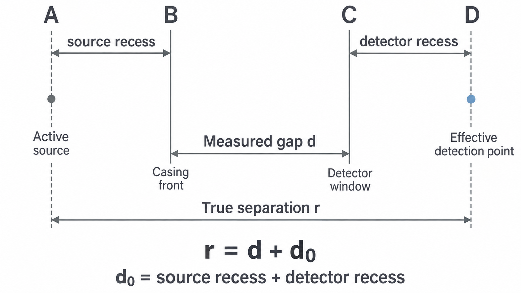
The sketch shows both the source recess and an effective detection region behind the window. The combined fixed offset $d_0$ includes both effects. The model uses $r=d+d_0$; do not identify $d_0$ with the source recess alone.

Measure a long background count with the source stored sufficiently far away and shielded. Record background total $N_b$ and time $t_b$. At each of several distances record the gross count $N$ and its actual time $t$. Pilot readings help choose a useful range and longer runs where the source signal is weak. Keep source orientation, detector voltage/settings and surrounding absorbers unchanged. Repeats check consistency; record unusual readings before deciding whether to repeat them.

Subtract rates, not totals taken over different times. A background of $180$ counts in $900\,\mathrm s$ gives $B=0.200\,\mathrm{s^{-1}}$. A source-present reading of $516$ counts in $120\,\mathrm s$ gives $C=4.30\,\mathrm{s^{-1}}$ and $C^{\prime}=4.10\,\mathrm{s^{-1}}$.

A suitable table records $d/\mathrm m$, $N$, $t/\mathrm s$, $C/\mathrm{s^{-1}}$, $C'/\mathrm{s^{-1}}$ and the transformed value with units. A spreadsheet can calculate these columns from the recorded raw values; inspect the formula in a sample row before filling it down. Save raw readings, settings and the source of the method so the analysis can be checked.

Linearising the true-distance model

A fixed distance offset changes which graph should be linear. With positive corrected rates,

Plot $y$ against measured $d$. The slope is $m=1/\sqrt K$, the vertical intercept is $b=d_0/\sqrt K$, and $d_0=b/m$. The horizontal intercept is $-d_0$. Since $C'$ has units $\mathrm{s^{-1}}$, $y$ has units $\mathrm{s^{1/2}}$ and $m$ has units $\mathrm{s^{1/2}\,m^{-1}}$.