3.13.3.1 - LC Resonance Filters
A parallel inductor–capacitor circuit can give a large response to a narrow range of frequencies. Follow its exchange of electrical and magnetic energy, calculate its resonant frequency, and use an energy or voltage response curve to decide whether a filter passes the wanted signal without admitting too much interference.
How a parallel LC circuit oscillates
A parallel LC circuit has an inductor of inductance , measured in henrys (H), and a capacitor of capacitance , measured in farads (F), connected across the same two nodes. An inductor opposes changes in current through an induced emf and stores energy in its magnetic field. A capacitor stores energy in its electric field.
[DIAGRAM: asset_name: parallel-lc-circuit; asset_slug: parallel-lc-circuit; caption: A charged capacitor connected in parallel with an inductor; description: Initial state of an isolated ideal LC circuit with capacitor upper plate positive, lower plate negative and zero current. Both components share the same two nodes.]
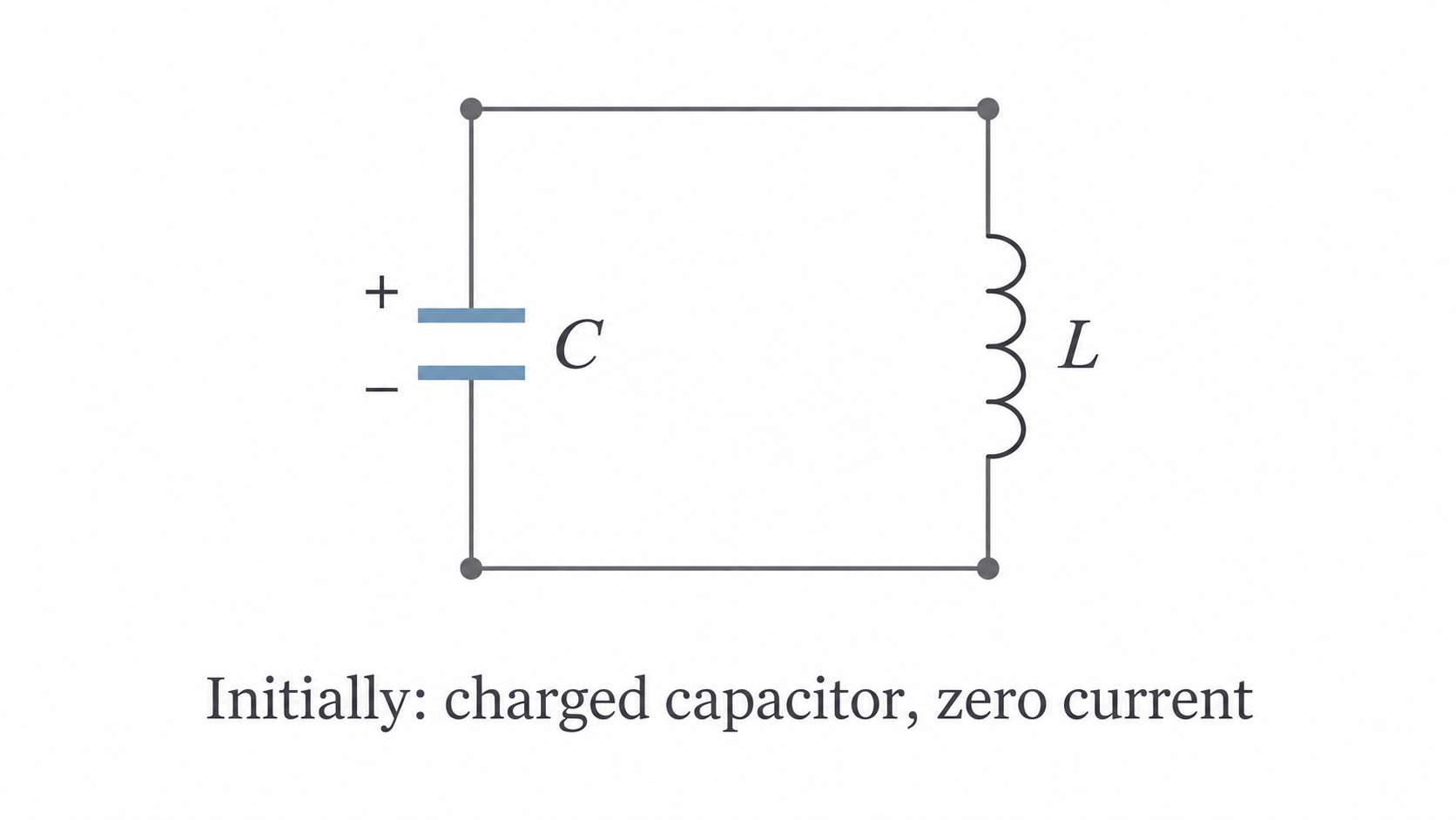
Imagine that the capacitor has been charged and its charging supply disconnected. Neglect resistance. The cycle then follows four stages:
| Stage | Capacitor | Inductor current and energy |
|---|---|---|
| Start | Maximum charge and voltage of one polarity | Zero current; all energy is electric |
| Quarter-cycle | Zero charge and voltage | Maximum current; all energy is magnetic |
| Half-cycle | Maximum charge with reversed polarity | Zero current; all energy is electric again |
| Three-quarter-cycle | Zero charge and voltage | Maximum current in the opposite direction; all energy is magnetic |
The original state returns after one complete cycle. The crucial quarter-cycle transition is that current continues in the same direction after the capacitor reaches zero charge. The inductor opposes the current's decrease; the capacitor therefore charges with the opposite polarity. Current reverses only after that reverse charge reaches its maximum and the current has fallen to zero.
The ideal total energy stays constant as its form changes. In a real coil and its leads, resistance transfers energy to the surroundings by heating, so the freely oscillating voltage decreases. This is damping. A driven circuit needs an external supply of energy to replace those losses.
The mass–spring analogy
An LC oscillator behaves like a mass attached to a spring: each system exchanges energy between two stores and overshoots its equilibrium state.
| Electrical quantity or behaviour | Mechanical counterpart |
|---|---|
| Charge on the capacitor | Displacement of the mass |
| Current , the rate of change of charge | Velocity , the rate of change of displacement |
| Inductance , opposing change of current | Mass , opposing change of velocity |
| Capacitance | Spring compliance , the inverse of stiffness |
| Capacitor electric energy | Spring elastic energy |
| Inductor magnetic energy | Mass kinetic energy |
| Energy loss in the coil/leads | Frictional damping |
At maximum displacement the mass is stationary, just as the fully charged capacitor has zero current. As the mass crosses equilibrium its speed is greatest, just as current is greatest when capacitor charge is zero. Inertia carries the mass through equilibrium; inductance maintains current through the instant of zero capacitor voltage.
A larger inductance is like a heavier mass, so changes occur more slowly. A larger capacitance stores more charge for a given voltage: it is like a softer spring, not a stiffer one. Both changes lower the natural frequency. The specification's “capacitance as spring” analogy should therefore be interpreted as capacitance corresponding to compliance, rather than to spring constant itself.
Calculating and tuning the resonant frequency
The inductance and capacitance set the natural frequency of an ideal LC oscillator and the approximate resonant frequency of a lightly damped parallel LC filter:
Parallel LC resonance
Use in henrys and in farads to obtain in hertz. Derivation is not required.
Increasing either or reduces . Quadrupling one component value halves the frequency because the product is under a square root. This agrees with the heavier-mass/softer-spring reasoning.
Worked tuning calculation
For and , convert both prefixes before substituting:
The final two significant figures match the component values. Keeping the intermediate value avoids rounding errors in later work.
To choose a capacitance for a specified station frequency, square and rearrange:
A variable capacitor lets a receiver move its response peak between station frequencies while the inductor stays fixed. Only parallel resonance arrangements are needed here.
Continue this lesson.
You’re previewing NovaLearn without an account. Create a free account to read the rest.
Create free account