3.11.2.3 - The p-V Diagram
Read pressure–volume paths, convert graphical area into signed work, and use loop direction to interpret the energy balance of a gas cycle.
Reading states and process paths
A pressure–volume diagram puts pressure on the vertical axis and volume on the horizontal axis. For a fixed amount of ideal gas, each equilibrium point also fixes temperature through . Arrows show which way the process runs.
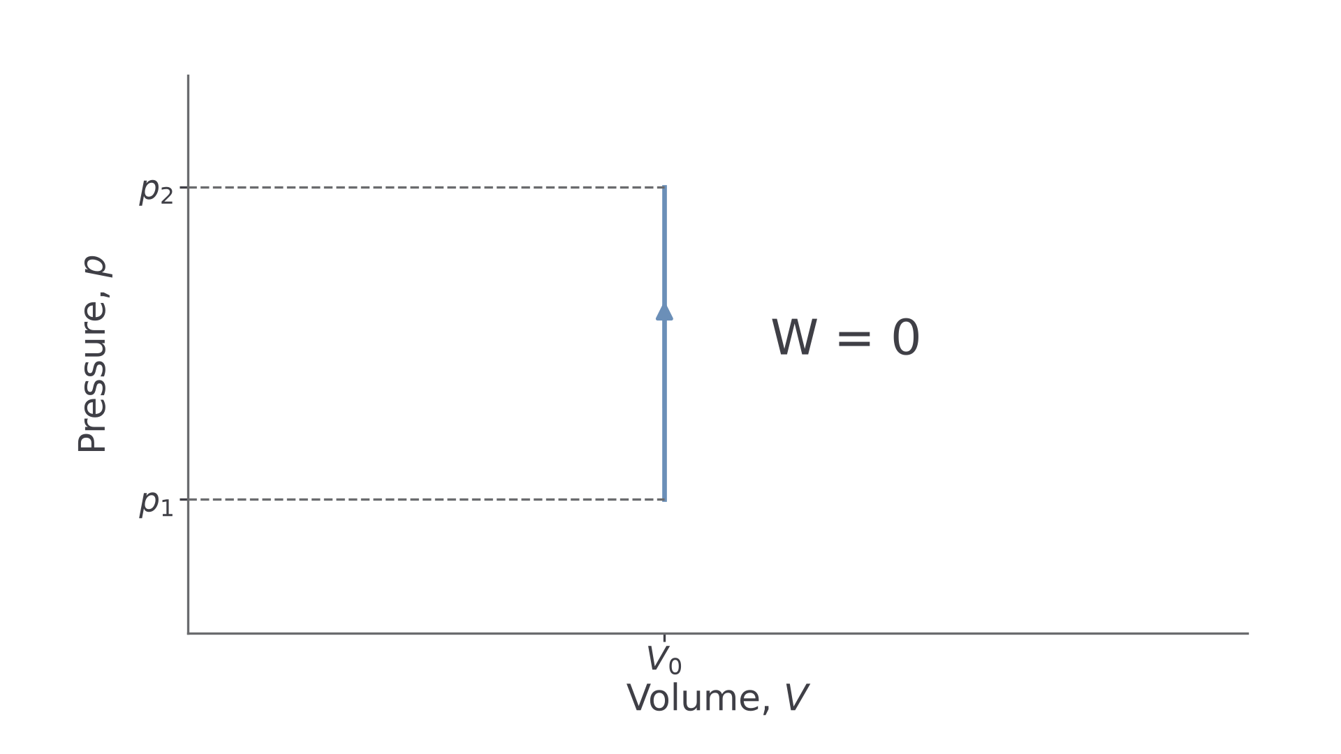
A horizontal path has constant pressure. A vertical path has constant volume: heating may raise pressure, but the boundary does not move.
[DIAGRAM: asset_name: C.2.3 - The p–V Diagram - Diagram 1; asset_slug: C.2.3 - The p–V Diagram - Diagram 1; caption: Constant-volume heating moves vertically upward. There is no horizontal width and no pressure–volume work.; description: Constant-volume heating moves vertically upward. There is no horizontal width and no pressure–volume work.]
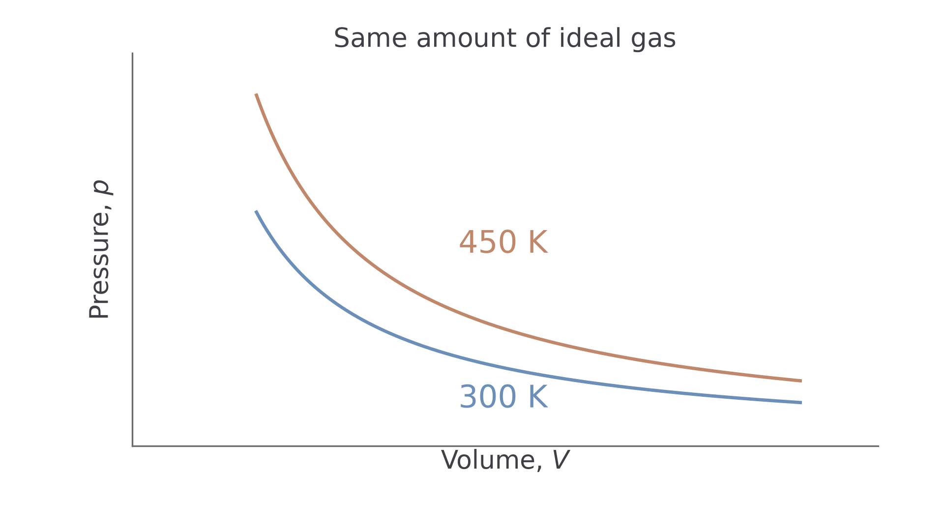
An isothermal ideal-gas path is a rectangular hyperbola, . For the same gas amount, higher temperature gives a higher pressure at every volume.
[DIAGRAM: asset_name: C.2.3 - The p–V Diagram - Diagram 2; asset_slug: C.2.3 - The p–V Diagram - Diagram 2; caption: The 450 K isotherm is above the 300 K isotherm for the same amount of ideal gas.; description: The 450 K isotherm is above the 300 K isotherm for the same amount of ideal gas.]
An adiabatic ideal-gas path follows . It is steeper than the isotherm at their common state, because expansion also cools the gas. Shape alone cannot prove a process is isothermal or adiabatic without scales, an equation or a stated thermal condition.
Area below a path is signed work
The work for a small volume change at approximately constant pressure is . Adding the narrow strips under a varying-pressure path gives its total work. Measure the area down to zero pressure, over only the volume interval traversed.
Expansion moves right and gives positive work by the gas. Compression moves left and gives negative work by the gas. A vertical line has zero width and therefore zero work.
[DIAGRAM: asset_name: C.2.3 - The p–V Diagram - Diagram 3; asset_slug: C.2.3 - The p–V Diagram - Diagram 3; caption: The shaded rectangle reaches the zero-pressure axis: constant-pressure work is p times the volume change.; description: The shaded rectangle reaches the zero-pressure axis: constant-pressure work is p times the volume change.]
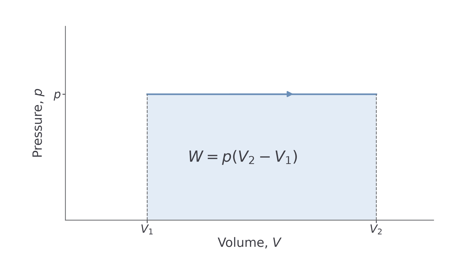
Check scale factors before measuring. Since , a square high and wide represents . Also , whereas .
For curved paths, estimate complete and partial squares or use trapezia. A strip with endpoint pressures and width has approximate work . Include every interval once. Narrower strips generally reduce approximation error; they do not remove uncertainty in the readings.
For instance, pressures at volumes give by two trapezia. AQA does not require memorised exact work expressions for curved paths.
Continue this lesson.
You’re previewing NovaLearn without an account. Create a free account to read the rest.
Create free account