3.4.2.1 - Bulk Properties of Solids

Density

A large object need not have a high density: density compares mass with volume, not mass alone. For a uniform material at a specified temperature,

Here $\rho$ is density in $\mathrm{kg\,m^{-3}}$, $m$ is mass in $\mathrm{kg}$ and $V$ is volume in $\mathrm{m^3}$. Doubling the amount of the same material doubles both mass and volume, leaving density unchanged. A hollow object's mass divided by its outer volume is its average density, which need not equal the density of the solid forming its walls.

Measure or estimate the volume

Measure mass on a zeroed balance. For a regular solid, measure its dimensions and use the appropriate geometry. A cylinder has $V=\pi d^2L/4$: the measured diameter must be halved if using $V=\pi r^2L$. For a non-porous irregular solid that does not dissolve, find volume from the increase in water level on complete immersion; remove trapped air and read the meniscus at eye level. For a rough estimate, approximate a shape by a cuboid or cylinder and state which dimensions were estimated.

A micrometer suits a small wire diameter; calipers suit a larger diameter; a rule suits a long length. A digital display avoids interpolation and some reading errors, but extra displayed digits do not guarantee greater accuracy: check resolution, zero error and instrument specification. Repeated dimensions reveal variation as well as reading scatter.

Keep the volume conversion cubic

Since $1\,\mathrm{cm}=10^{-2}\,\mathrm m$, $1\,\mathrm{cm^3}=10^{-6}\,\mathrm{m^3}$. Thus $1\,\mathrm{g\,cm^{-3}}=1000\,\mathrm{kg\,m^{-3}}$.

For a steel cylinder of diameter $12\,\mathrm{mm}$ and length $85\,\mathrm{mm}$,

If $\rho=7800\,\mathrm{kg\,m^{-3}}$, its mass is $m=\rho V=0.0750\,\mathrm{kg}$. Using metres before squaring prevents a factor-of-a-million volume error.

Hooke's Law and the Spring Constant

Stretching a spring requires a force whose size may change as the spring extends. Extension $x=\Delta L$ is the increase from the natural length, not the final length.

Within the limit of proportionality, force is directly proportional to extension. The constant $k$, in $\mathrm{N\,m^{-1}}$, measures the stiffness of this particular object: a larger $k$ means more force for the same extension. This equation uses force magnitudes; a restoring force on a displaced object acts opposite to its displacement.

A graph of force vertically against extension horizontally is straight through the origin while Hooke's law holds. Its gradient is $k=\Delta F/\Delta x$. If the axes are reversed, the gradient is $1/k$.

[DIAGRAM: asset_name: 4.2.1 - Bulk Properties of Solids - Diagram 1; asset_slug: 4.2.1 - Bulk Properties of Solids - Diagram 1; caption: Proportionality limit P and elastic limit E on an illustrative force–extension curve; description: Force vertically in N against extension horizontally in m. Initial line from origin ends at P. Curve continues through E.]

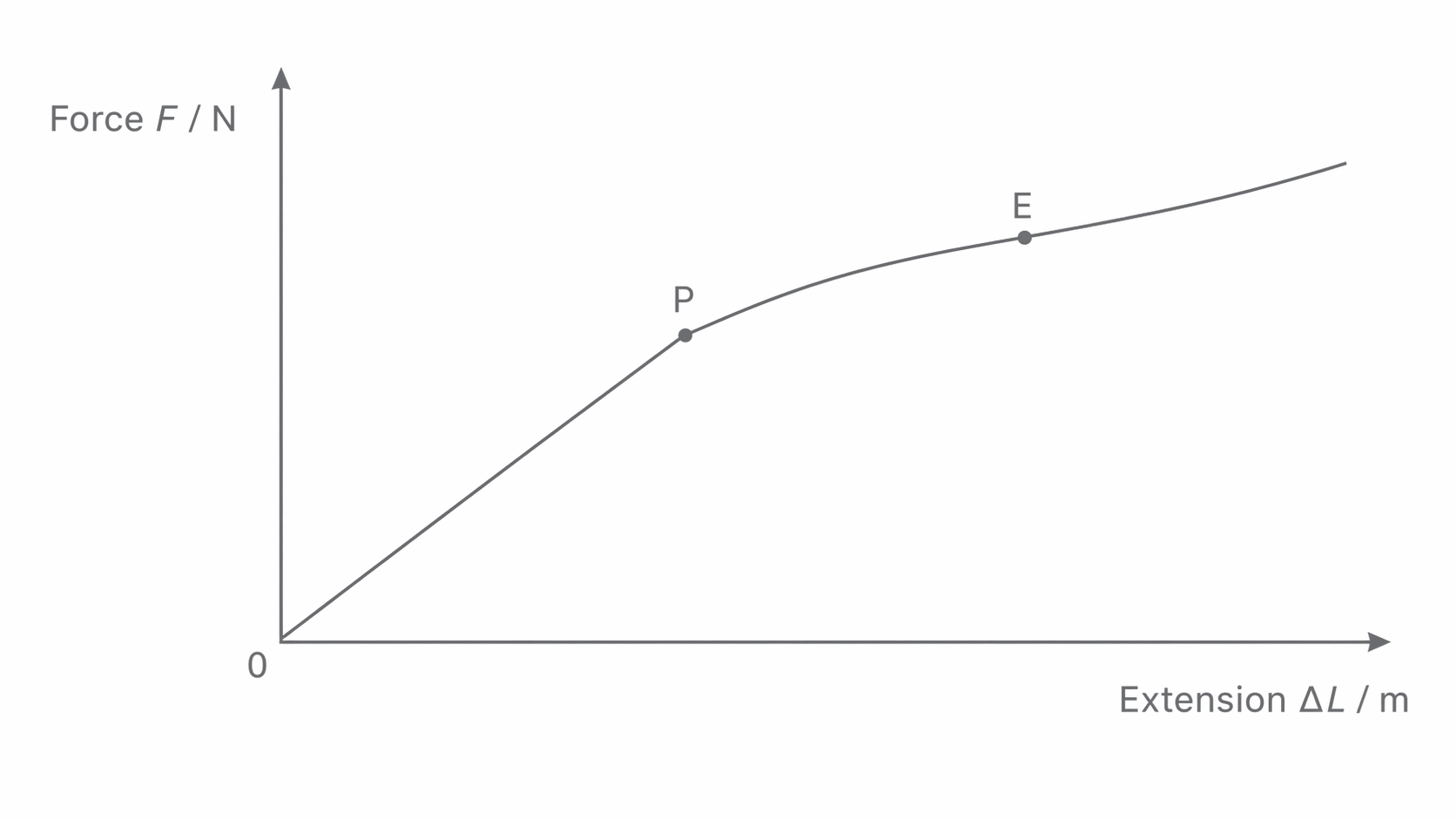
The point $P$ marks the end of direct proportionality. The elastic limit, labelled $E$ here, is the greatest loading from which the object returns to its original length when unloaded. These limits need not coincide: between them a material can be elastic but non-linear. Their separation varies between materials. A loading curve locates the proportionality limit, but unloading measurements are needed to establish the elastic limit.

Tensile Stress and Tensile Strain

Two wires made from the same material can have different force–extension graphs because their dimensions differ. Tensile stress accounts for area and tensile strain accounts for original length, allowing a fairer comparison.

Stress $\sigma$ is tensile force per unit original cross-sectional area, in pascals: $1\,\mathrm{Pa}=1\,\mathrm{N\,m^{-2}}$. For a circular wire $A=\pi d^2/4$. The force on each end has magnitude $F$; do not add the opposite pulls to make $2F$.

Strain $\varepsilon$ is extension divided by original length. Both lengths must use the same unit, so strain has no unit. A $2.0\,\mathrm{mm}$ extension on a $2.0\,\mathrm m$ wire gives $\varepsilon=0.0010$, or $0.10\%$, not $1.0\%$.

For a $0.30\,\mathrm{mm}$ diameter wire under $6.0\,\mathrm N$,

Halving the diameter at the same force makes the area one-quarter as large and the stress four times larger. A longer wire under the same stress can extend more while having the same strain. Samples of the same uniform material in the same condition and temperature have comparable stress–strain behaviour; composition, heat treatment and damage can change it.

Elastic Strain Energy

A force does work while its point of application moves. During a small extra extension the work is approximately force multiplied by that extra extension. Adding these contributions gives the area under a force–extension graph.

For loading from zero force to force $F$ along a straight line through the origin, the mean force is $F/2$. The triangular area is

Use extension in metres so that the area is in $\mathrm{N\,m}=\mathrm J$. The formula assumes proportional loading and negligible dissipation; merely saying that the object eventually returns to its original shape does not establish a straight-line graph.

If a spring with $k=120\,\mathrm{N\,m^{-1}}$ extends by $0.050\,\mathrm m$, it stores $0.150\,\mathrm J$. Doubling extension doubles the final force and doubles the graph's base, so energy becomes four times greater.

Loading work and recovered energy

For a non-linear material, find area under the actual curve by counting squares, splitting it into strips or using supplied numerical areas. The area under the loading path is work put into the material. Area under the unloading path is energy returned mechanically. Their difference is energy not returned, commonly transferred to internal energy. A hysteresis loop can occur even if the material eventually regains its initial length, as with rubber; elastic return does not guarantee loss-free behaviour.

Plastic, Brittle, and Ductile Behaviour

The shape left after unloading distinguishes elastic from plastic deformation. Elastic deformation is reversed; plastic deformation leaves a permanent change of length or shape. A curved loading graph alone does not distinguish them.

[DIAGRAM: asset_name: 4.2.1 - Bulk Properties of Solids - Diagram 2; asset_slug: 4.2.1 - Bulk Properties of Solids - Diagram 2; caption: Unloading after plastic deformation leaves permanent extension and returns less energy; description: Illustrative force–extension loading curve with an unloading line returning to nonzero extension. Shading is loading work minus recovered work.]

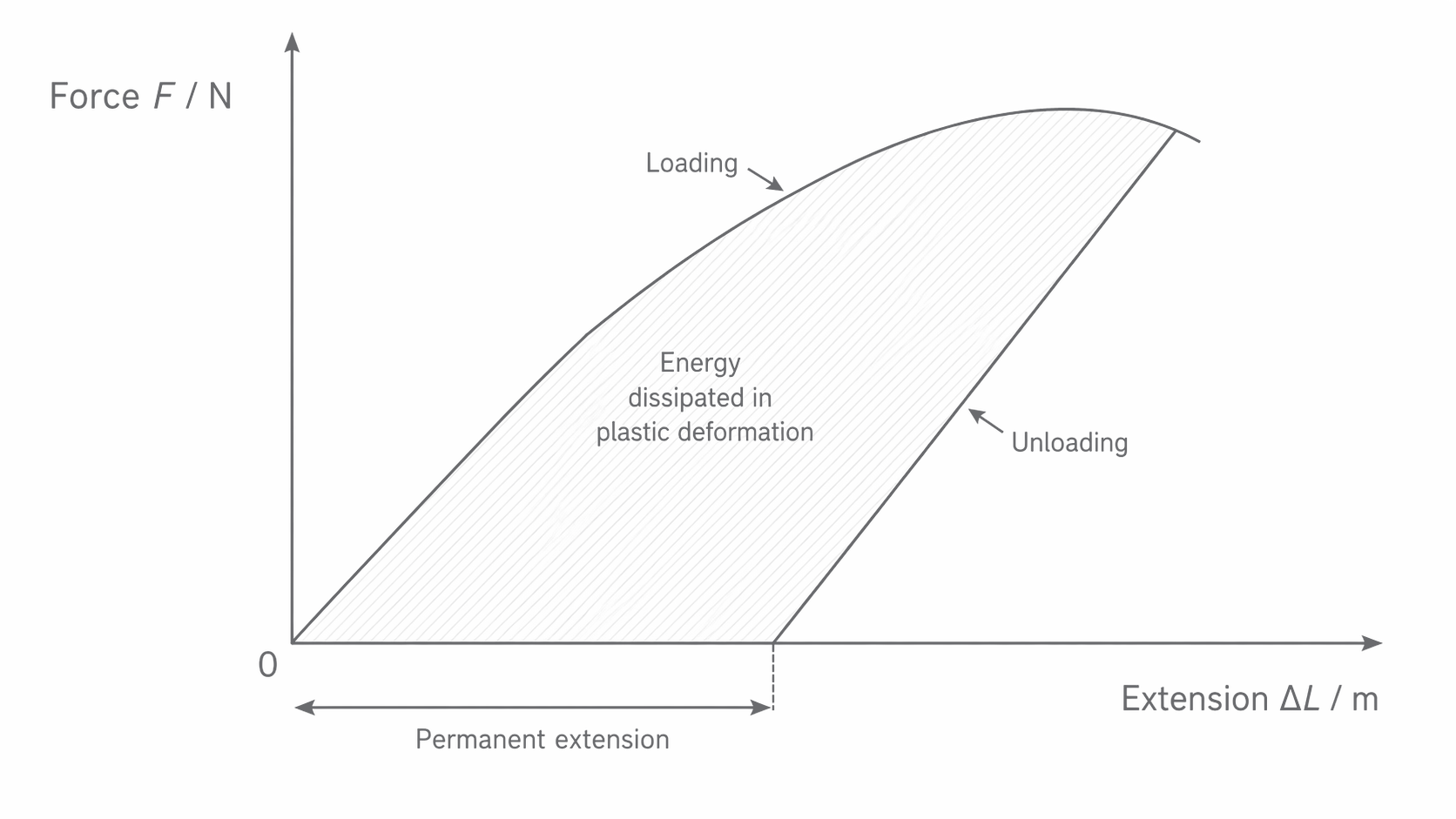
In this illustration unloading begins at the chosen high-load point, before the loading curve's far-right end. The unloading path reaches zero force at a positive extension: the wire has become permanently longer. Its slope is often close to the original elastic slope, but exact parallelism is not the test for plastic behaviour. The shaded difference in areas represents energy not returned mechanically; the triangle under the unloading line is the energy recovered.

Yielding describes the onset of appreciable plastic flow: a relatively large extra strain occurs for little increase in stress. Some materials have a clear yield point or plateau, while others yield gradually. Do not label every bend as a distinct yield point.

A brittle material fractures with little or no plastic deformation. Its graph often has an approximately straight elastic section ending abruptly at fracture. A ductile material undergoes substantial plastic strain before fracture and can be drawn into a wire. Brittleness does not, by itself, specify the initial gradient or the breaking stress.

[DIAGRAM: asset_name: 4.2.1 - Bulk Properties of Solids - Diagram 3; asset_slug: 4.2.1 - Bulk Properties of Solids - Diagram 3; caption: Illustrative brittle and ductile stress–strain curves ending at fracture; description: Stress in Pa vertically and dimensionless strain horizontally. The illustrated brittle sample ends at small strain. The ductile sample yields and accumulates much greater strain before fracture.]

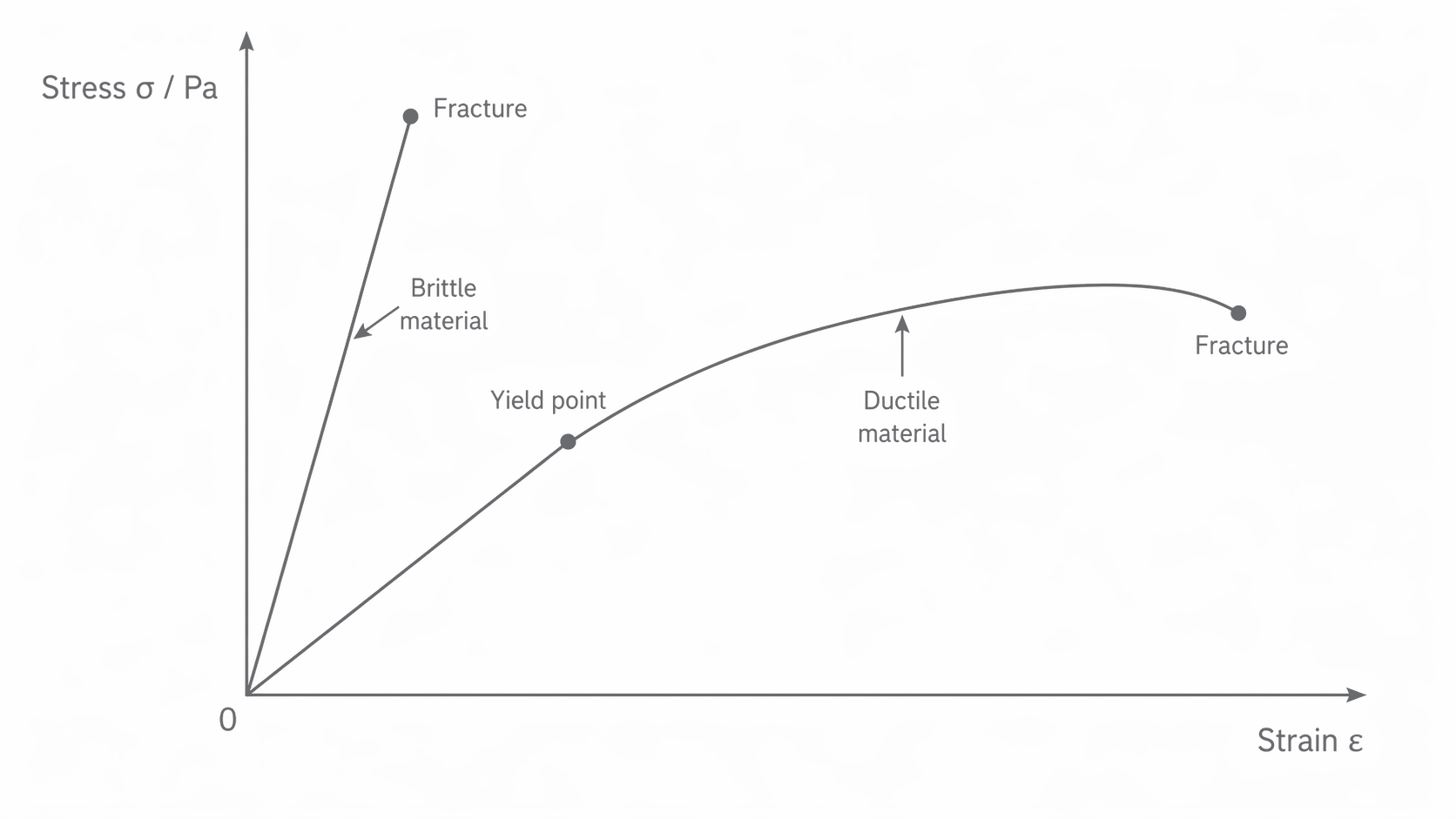
The illustrated brittle sample has the steeper initial gradient and higher fracture stress; that ordering is not universal. Breaking stress is tensile force at fracture divided by original cross-sectional area: read the stress at the final point. If the curve first rises to a peak and then falls, the peak stress and breaking stress differ. A design needs an adequate safety margin against both permanent deformation and fracture.

Spring Energy and Transport Design

Energy conservation connects the work used to deform a material with the motion it can produce or stop. Choose initial and final states, then include every energy store that changes between them.

A spring launcher

A horizontal spring with $k=150\,\mathrm{N\,m^{-1}}$ compressed by $0.040\,\mathrm m$ stores $0.120\,\mathrm J$. If a $0.012\,\mathrm{kg}$ dart leaves at the natural length, with negligible losses and spring mass,

If the launcher points vertically, the dart gains gravitational potential energy while the spring expands. At loss of contact after rising $x$,

Alternatively, compare the compressed start directly with the highest point: $\tfrac12kx^2=mg\Delta h$, where $\Delta h$ is the total rise from the starting position. For the same dart, $\Delta h=0.120/(0.012\times9.81)=1.02\,\mathrm m$. Height gained above the natural-length position is $1.02-0.040=0.98\,\mathrm m$. Any energy dissipated must be included separately and reduces these ideal predictions.

Why a car is allowed to crumple

During a crash the car loses kinetic energy. Plastic deformation transfers some of that energy into internal energy and lasting structural change rather than returning it as rebound. For a given energy transfer $W$, increasing the stopping distance $s$ lowers average stopping force because $F_{\mathrm{avg}}=W/s$. The corresponding impulse argument is that a longer stopping time reduces average force for the same momentum change.

A crumple zone must deform in a controlled way while the passenger compartment remains protective; simply using the weakest material is not sufficient. Restraints also need to slow occupants over a suitable distance. Ethical design balances occupant and pedestrian safety, repair cost, material use and environmental impact. Extra mass can increase both crash energy at a given speed and energy used during transport, so a claim that a heavier design is automatically safer is inadequate.