3.7.3.3 - Electric Potential

Potential and its zero reference

Absolute electric potential at a point is the external work done per unit positive test charge in bringing a small positive test charge from infinity to that point without changing its kinetic energy. The charge is moved slowly so that the work measures potential-energy change. The test charge is small enough not to disturb the sources.

With the zero of potential at infinity, $V=E_\mathrm{p}/q$, where $E_\mathrm{p}$ is the test charge's electric potential energy relative to infinity. One volt is one joule per coulomb: $1\,\mathrm{V}=1\,\mathrm{J\,C^{-1}}$. Potential is a property of position in the source field; potential energy also depends on the charge placed there, through $E_\mathrm{p}=qV$.

Potential is a scalar: its positive or negative sign is not a spatial direction. Near an isolated positive source, bringing a positive test charge inward requires positive external work against repulsion, so the potential is positive. Near an isolated negative source, the field attracts the positive test charge inward; a slow external mover removes energy, so its work and the potential are negative.

The infinity reference is appropriate for isolated finite source distributions. Potential differences are independent of the chosen zero: adding the same constant to every potential leaves both $\Delta V$ and the field unchanged. A plate supply normally specifies a difference, not an absolute potential relative to infinity.

Energy changes and work signs

A charge moving from A to B has signed potential change $\Delta V=V_\mathrm{B}-V_\mathrm{A}$. Use the actual sign of the moving charge in the energy equation:

For slow external movement with no kinetic-energy change, $W_\mathrm{external}=q\Delta V$. For free motion under only the electric force, $\Delta K=W_\mathrm{field}=-\Delta E_\mathrm{p}$. These statements specify who does the work; the phrase “work done” alone can conceal a sign error.

An electron, $q=-1.60\times10^{-19}\,\mathrm{C}$, moves from $-50\,\mathrm{V}$ to $+450\,\mathrm{V}$. Here $\Delta V=+500\,\mathrm{V}$, giving $\Delta E_\mathrm{p}=-8.0\times10^{-17}\,\mathrm{J}$. The field does $+8.0\times10^{-17}\,\mathrm{J}$ of work. If other energy transfers are negligible, the electron gains that much kinetic energy. A negative charge can therefore gain kinetic energy while moving to higher potential; it still moves towards lower potential energy.

In an electrostatic field these energy changes depend only on the endpoints, not on the route. If a positive charge goes around a closed path back to the same potential, the net field work is zero, even though individual stages can involve nonzero work.

Equipotentials and perpendicular fields

An equipotential surface has the same potential at every point. Moving charge along it gives $\Delta V=0$, hence no change in electric potential energy and no work by the electric field. This does not say that every force acting on the object does zero work; it refers to the electric interaction.

Where the field is nonzero, it is perpendicular to an equipotential surface. If the field had a component along the surface, the electric force would do work during motion along it, contradicting $\Delta V=0$. In a uniform plate field the surfaces are parallel planes. For an isolated point charge they are concentric spheres, shown as circles in a cross-section.

[DIAGRAM: asset_name: 7.3.3 - Electric Potential - Diagram 1; asset_slug: 7.3.3 - Electric Potential - Diagram 1; caption: Equal potential steps are equally spaced in a uniform field but spread out in a radial field; description: Exact plane and circular equipotential geometry with numerical values. Field arrows cross contours normally and point towards decreasing potential.]

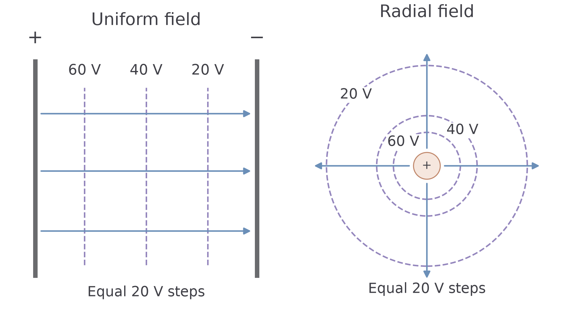
Only contours chosen at equal potential intervals can be used directly to compare field strengths from spacing. In the radial example, $V=12/r$ with SI units: $60$, $40$ and $20\,\mathrm{V}$ occur at $0.20$, $0.30$ and $0.60\,\mathrm{m}$. Equal $20\,\mathrm{V}$ drops require increasing distances outward, showing that the field becomes weaker. A set of arbitrarily chosen equipotentials need not display this spacing rule.

A charge moved around a circle centred on the isolated source can have nonzero force throughout, yet zero electric work: at each point the radial force is perpendicular to its tangential displacement. Zero work along a path does not imply zero field.

Potential around a point charge

For an isolated point source $Q$, with zero potential at infinity,

Use signed $Q$. The potential has the same sign as the source charge, while its magnitude varies as $1/r$. Positive-source potential approaches zero from above with increasing distance; negative-source potential approaches zero from below. Outside a spherically symmetric charged sphere the same expression applies with distance measured from its centre.