RP09 - Capacitor Charge and Discharge
Investigate capacitor charging and discharging, turn voltage readings into log-linear plots, and determine the time constant with justified uncertainty. RP09 is the course label for AQA required practical 9.
Exponential models and their linear forms
The required investigation measures capacitor pd during charging and discharging and uses log-linear analysis to determine . With constant , negligible meter loading and leakage, and a constant source emf ,
Here discharge starts at , while charging starts from zero. The time constant is the time for discharge pd to fall to 36.8% of its initial value, or charging pd to rise to 63.2% of its final value. Current decreases in magnitude in both cases. The capacitor's positive plate stays positive while discharging; current reverses relative to charging at that terminal.
Taking a natural logarithm of a dimensionless voltage ratio gives a straight-line form:
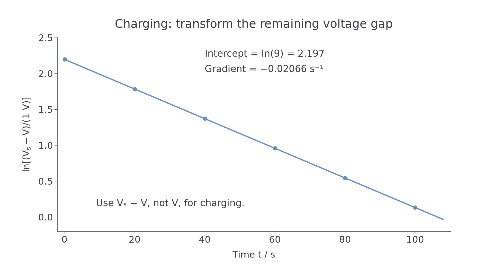
Both plots against have gradient , so . A shorthand such as 'ln V' means the logarithm of the numerical voltage in a specified unit. For charging, plot the remaining voltage gap, not . A straight line supports the exponential model over the measured range; it does not prove the components ideal.
A circuit that measures both processes
A single-pole double-throw switch can put the same resistor in the charging and discharging paths. Connect its common terminal to the resistor, then to the capacitor's positive terminal. Contact A connects to the supply positive terminal; contact B connects to the common negative return. The capacitor negative terminal and supply negative terminal share that return. A high-input-resistance voltmeter is connected across the capacitor.
[DIAGRAM: asset_name: RP 09 - Investigation of the Charge and Discharge of Capacitors - Diagram 1; asset_slug: RP 09 - Investigation of the Charge and Discharge of Capacitors - Diagram 1; caption: The switch common terminal connects to R. A connects to the positive supply to charge, B connects to the negative return to discharge through the same R while isolating the supply positive terminal. The voltmeter is across C.; description: The switch common terminal connects to R. A connects to the positive supply to charge, B connects to the negative return to discharge through the same R while isolating the supply positive terminal. The voltmeter is across C.]
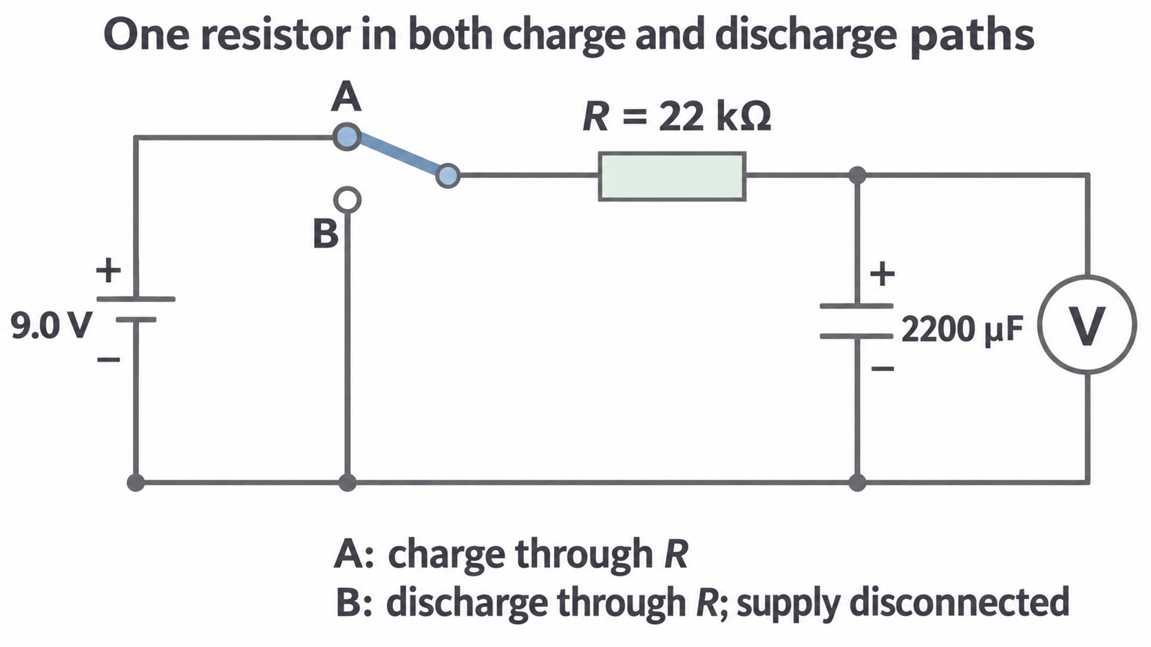
Suitable example values are , and a supply. Their nominal is slow enough for readings every 5–10 s and a run lasting a few minutes. Use actual measured values and manufacturer tolerances where available, not the label as an exact value.
Check electrolytic polarity and use a capacitor voltage rating above the supply. The resistor limits current in both positions. Its maximum initial power here is , comfortably below a rating. Discharge through a resistor before handling/reconnecting; do not short the terminals as a discharge method.
Recording a run
- With the supply off, check connections, polarity and meter range. Measure with power disconnected and the capacitor safely discharged.
- For discharge, set A and wait roughly until the pd is steady. Record that actual initial pd.
- Move to B and begin timing together. Record at regular intervals across several time constants. A trial run helps choose intervals and a usable lower-voltage limit.
- Recharge to the same initial pd and repeat complete runs. Compare readings at common times; use their mean and scatter.
- For charging, first leave the switch at B until the capacitor pd is negligible. Move to A and record the rise from zero. Measure the final steady pd for the logarithmic transform.
A data logger with a voltage sensor records and timestamps together. Choose an interval much shorter than and record long enough to see the asymptote; synchronise the switching event or identify it in the recording. Logging reduces manual reaction/readout errors, but still has sampling, trigger and sensor uncertainties. For rapid changes an oscilloscope with a suitable square-wave source is an alternative.
Controls, range and a fair comparison
Time is the independent variable within each run and capacitor pd is the dependent variable. Keep the same resistor, capacitor, circuit and temperature between repeats. Reproduce the initial charge state and use a stable supply for charging. For ideal discharge, a changed starting pd changes the intercept but does not change ; it does not itself destroy exponential behaviour.
Use a preliminary run to choose enough points to resolve the early change and span a broad range of the decay. A fixed minimum count is not a substitute for useful range and sensible uncertainty. Near zero discharge voltage, a fixed meter uncertainty becomes a large fraction of the reading. During charging, the same problem occurs when becomes small. Stop or down-weight unsuitable points for a stated measurement reason; do not remove inconvenient points merely to make a straight line.
Repeats reveal scatter and allow a mean, reducing the effect of random errors. They do not remove calibration error, leakage or meter loading. Record instrument resolution, any manufacturer accuracy specification and observed repeat variation. Repeated identical display values do not justify zero uncertainty or uncertainty smaller than the relevant instrument limit.
A useful comparison tests measured against independently measured with uncertainty. A capacitor tolerance is a permitted range around its marked value; being different from the marking does not by itself show a faulty method. Straightness tests the model, while agreement of time constants tests the parameter values—these are separate judgements.
Processing charging and discharging data
The following original simulated readings illustrate the processing for and . They are rounded model values, not claimed laboratory or AQA handbook measurements.
Here is the discharging pd and the charging pd. The final column gives both transformed values: and . They are equal for this matched pair of runs.
| 0 | 9.00 | 0.00 | 2.197 |
| 20 | 5.95 | 3.05 | 1.783 |
| 40 | 3.94 | 5.06 | 1.371 |
| 60 | 2.61 | 6.39 | 0.959 |
| 80 | 1.72 | 7.28 | 0.542 |
| 100 | 1.14 | 7.86 | 0.131 |
[DIAGRAM: asset_name: RP 09 - Investigation of the Charge and Discharge of Capacitors - Diagram 2; asset_slug: RP 09 - Investigation of the Charge and Discharge of Capacitors - Diagram 2; caption: Model charging and discharging curves for V0 = 9.00 V and RC = 48.4 s. At one time constant their voltages are 5.69 V and 3.31 V respectively.; description: Model charging and discharging curves for V0 = 9.00 V and RC = 48.4 s. At one time constant their voltages are 5.69 V and 3.31 V respectively.]
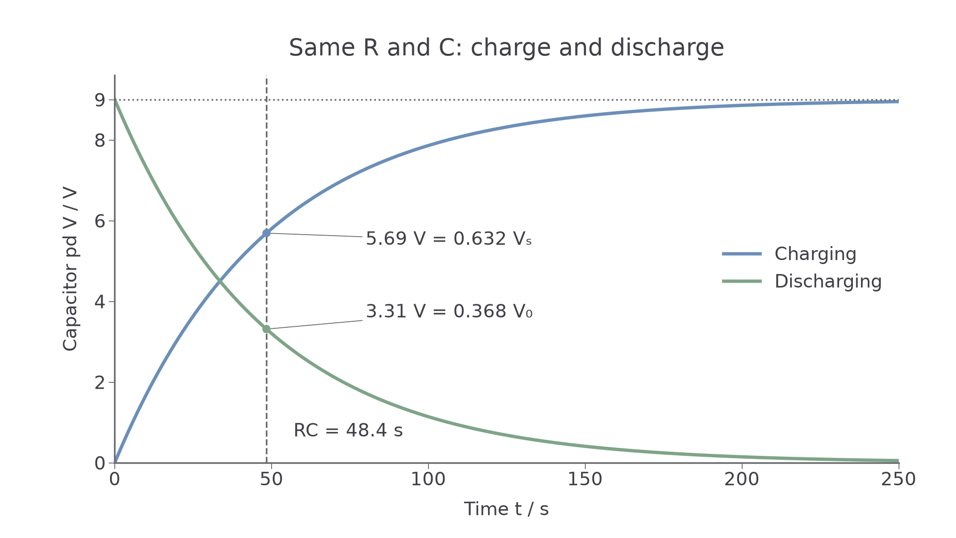
Transform each positive discharge voltage, or each positive charging gap. is undefined. A reading apparently equal to the final supply voltage reflects finite resolution; it cannot be plotted as a logarithm of zero. Use the measured asymptote: an incorrect can create curvature in the charging transform, especially late in the run.
[DIAGRAM: asset_name: RP 09 - Investigation of the Charge and Discharge of Capacitors - Diagram 4; asset_slug: RP 09 - Investigation of the Charge and Discharge of Capacitors - Diagram 4; caption: The charging voltage gap Vs - V decays exponentially. For the same model as the raw curves, ln[(Vs - V)/(1 V)] is linear with gradient -1/48.4 per second and intercept ln(9).; description: The charging voltage gap Vs - V decays exponentially. For the same model as the raw curves, ln[(Vs - V)/(1 V)] is linear with gradient -1/48.4 per second and intercept ln(9).]
Continue this lesson.
You’re previewing NovaLearn without an account. Create a free account to read the rest.
Create free account