3.4.1.3 - Motion Along a Straight Line

Position, velocity and acceleration

Choose an origin and a positive direction before describing motion. Displacement is change in position, not total path length. Average velocity is displacement divided by elapsed time, whereas average speed is total distance divided by elapsed time.

Velocity has units $\mathrm{m\,s^{-1}}$, and acceleration has units $\mathrm{m\,s^{-2}}$. The equations above give averages over an interval. Instantaneous velocity and acceleration refer to a particular instant; they are found from a tangent on the appropriate graph.

A runner goes $60\,\mathrm{m}$ east then $20\,\mathrm{m}$ west in $16\,\mathrm{s}$. Average velocity is $+2.5\,\mathrm{m\,s^{-1}}$, with east positive, but average speed is $5.0\,\mathrm{m\,s^{-1}}$.

Acceleration describes change in velocity, not speed alone. If velocity and acceleration have the same sign, speed increases. If their signs differ, speed decreases. A negative acceleration can therefore speed up an object travelling in the negative direction.

Reading gradients and signed areas

The gradient of a displacement–time graph is velocity. A horizontal section means rest; a downward slope means negative velocity. A changing gradient means changing velocity. To estimate instantaneous velocity, draw a tangent and choose two well-separated points on that tangent, not two points on the curve.
[DIAGRAM: asset_name: 4.1.3 - Motion Along a Straight Line - Diagram 1; asset_slug: 4.1.3 - Motion Along a Straight Line - Diagram 1; recommended_method: retained_png; caption: A numerical displacement–time graph: the tangent at 6 s has gradient 4 m s⁻¹, the interval-average velocity need not equal it.; description: A numerical displacement–time graph: the tangent at 6 s has gradient 4 m s⁻¹, the interval-average velocity need not equal it.]

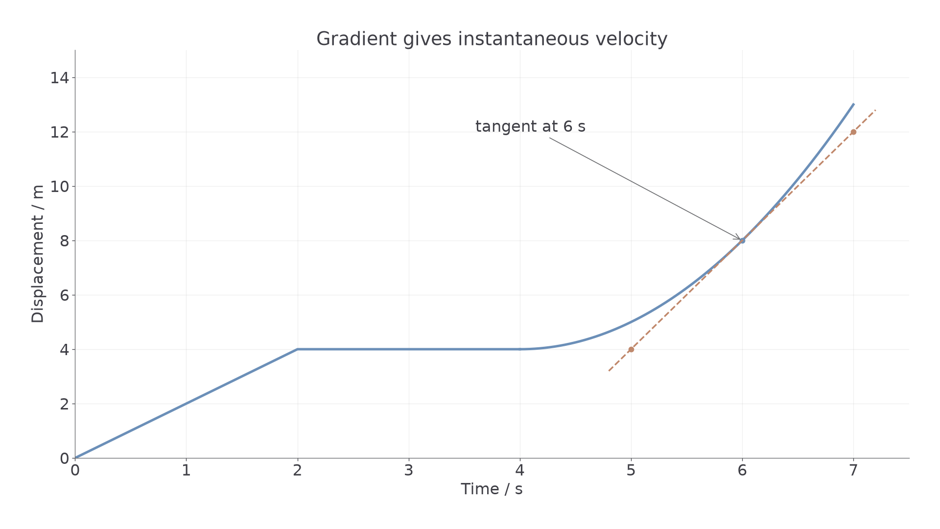
On this graph, displacement rises from 0 to $4\,\mathrm{m}$ in 2 s, stays at 4 m until 4 s, then follows $s=4+(t-4)^2$. At 6 s, the tangent passes through $(5,4)$ and $(7,12)$, so instantaneous velocity is $4\,\mathrm{m\,s^{-1}}$. Average velocity from 4 to 7 s is $(13-4)/3=3\,\mathrm{m\,s^{-1}}$.

The gradient of a velocity–time graph is acceleration. Straight slopes mean constant acceleration; a curve means changing acceleration, found locally from a tangent. A downward slope does not automatically mean slowing down: below zero it can mean increasingly negative velocity and increasing speed.

The signed area between velocity and the time axis gives displacement. Add positive areas and subtract negative areas. For total distance, add the magnitudes of all areas and split any section where it crosses zero.
[DIAGRAM: asset_name: motion-signed-areas; asset_slug: motion-signed-areas; recommended_method: retained_png; caption: Signed velocity–time areas give displacement, their magnitudes give distance. The matching acceleration graph gives change in velocity.; description: Signed velocity–time areas give displacement, their magnitudes give distance. The matching acceleration graph gives change in velocity.]

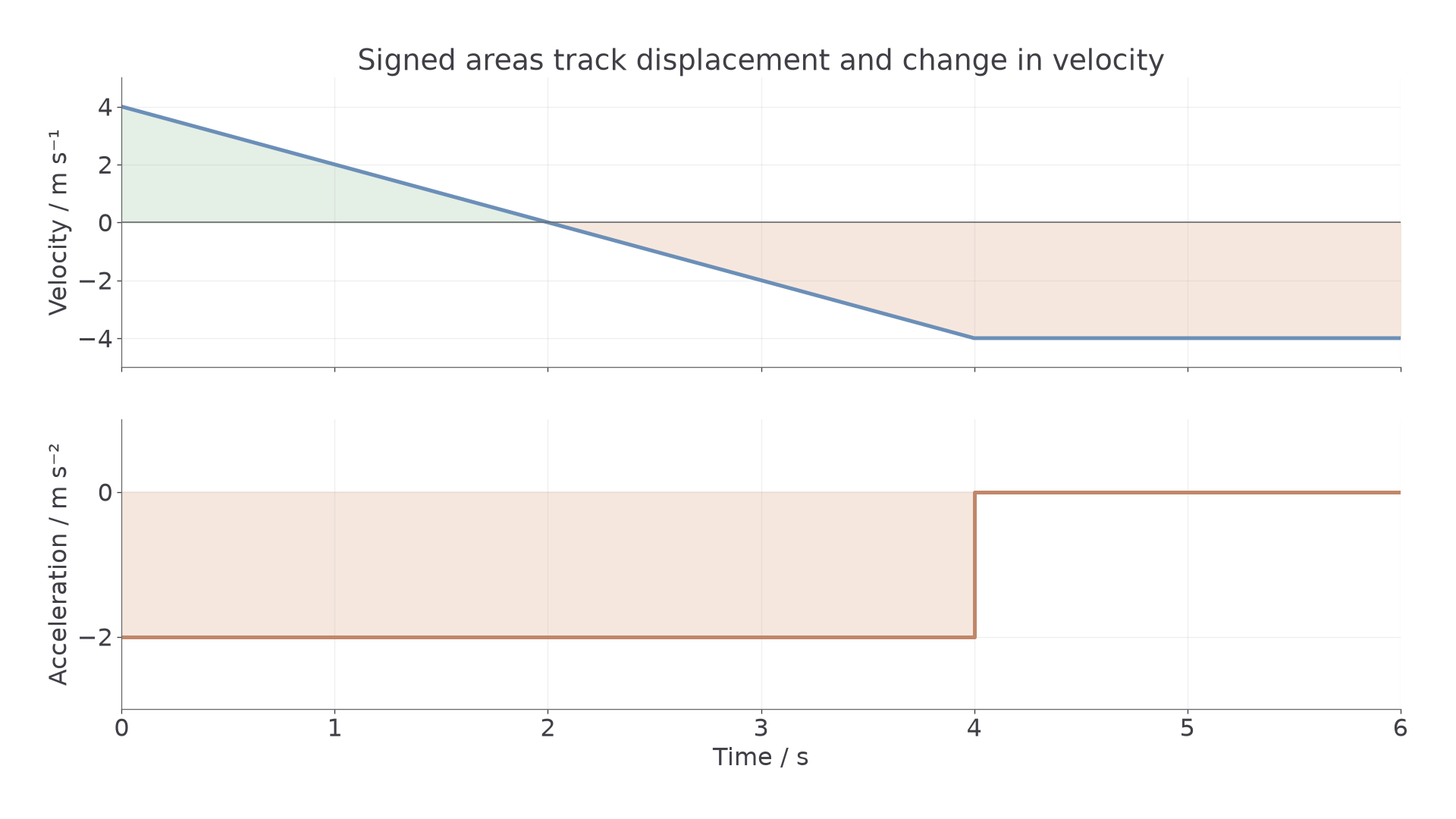
Here the velocity falls from $+4$ to $-4\,\mathrm{m\,s^{-1}}$ in 4 s, then stays at $-4$ until 6 s. The first positive triangle is $+4\,\mathrm{m}$, the next is $-4\,\mathrm{m}$, and the rectangle is $-8\,\mathrm{m}$. Displacement is $-8\,\mathrm{m}$; distance is $16\,\mathrm{m}$.

The signed area under an acceleration–time graph is change in velocity, not velocity itself. In this example $\Delta v=(-2)(4)+0(2)=-8\,\mathrm{m\,s^{-1}}$; adding the initial $+4$ gives final velocity $-4$. For curved graphs, estimate areas using narrow trapezia and gradients using tangents; do not assume constant acceleration over the whole curve.
[DIAGRAM: asset_name: motion-nonuniform; asset_slug: motion-nonuniform; recommended_method: retained_png; caption: A curved velocity graph has changing gradient. Tangents and acceleration areas describe the same changes in velocity.; description: A curved velocity graph has changing gradient. Tangents and acceleration areas describe the same changes in velocity.]

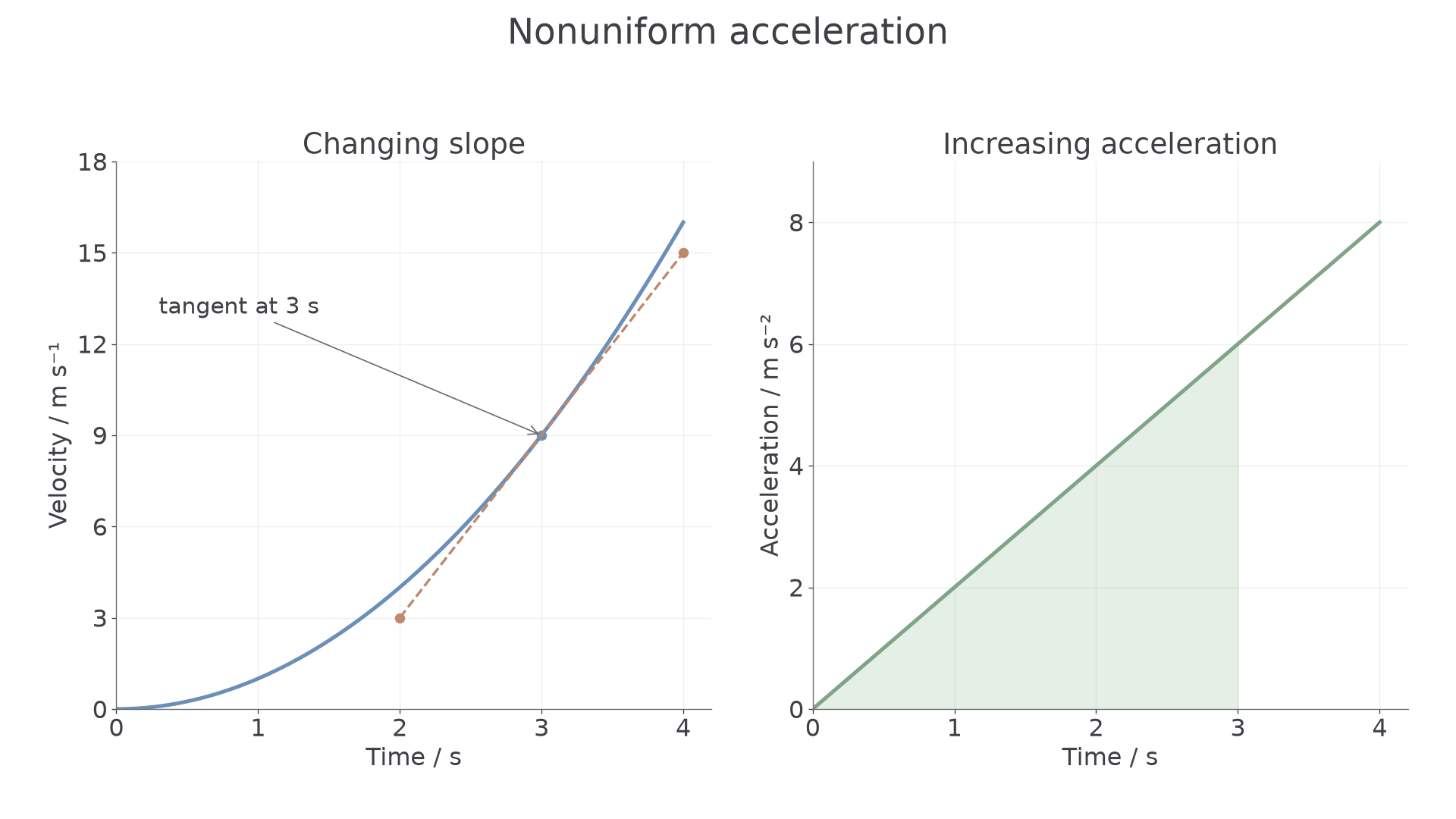
For the nonuniform example, velocity rises as $v=t^2$ when the numerical values are in SI units. The tangent at 3 s passes through $(2,3)$ and $(4,15)$, giving instantaneous acceleration $(15-3)/(4-2)=6\,\mathrm{m\,s^{-2}}$. This exceeds the average acceleration from 0 to 3 s, $(9-0)/3=3\,\mathrm{m\,s^{-2}}$. The acceleration graph's triangular area from 0 to 3 s is $\tfrac12(3)(6)=9\,\mathrm{m\,s^{-1}}$, matching the velocity change. A single constant-acceleration equation would not describe this whole interval.

Deriving constant-acceleration equations

For constant acceleration, the velocity–time graph is a straight line. Let $u$ and $v$ be its initial and final velocities, $t$ the elapsed time, and $s$ the displacement. Its gradient and signed trapezium area give

Substituting $v=u+at$ into the area expression gives

Eliminating time instead, using $t=(v-u)/a$ when $a\ne0$, gives

The last equation also holds for $a=0$; it then states $v^2=u^2$ and cannot determine displacement. Squaring a velocity loses its sign, so choose the physically correct sign when taking a square root.

The four equations are algebraically related, not four independent physical laws. Each omits a different variable, allowing a convenient route without an unnecessary intermediate calculation. They do not describe a whole interval of changing acceleration, though separate constant-acceleration stages can be treated individually.

Choosing equations and linking stages

List known quantities with signs, select an equation that omits the unused unknown, and interpret the result physically. Keep unrounded values until the final answer.

A car braking uniformly from $30\,\mathrm{m\,s^{-1}}$ to rest over $100\,\mathrm{m}$, with forward positive, obeys

The acceleration is negative; the deceleration magnitude is $4.5\,\mathrm{m\,s^{-2}}$.

For a two-stage journey, the final velocity of one continuous stage becomes the initial velocity of the next. A cyclist accelerates from rest at $0.40\,\mathrm{m\,s^{-2}}$ for $20\,\mathrm{s}$: $v=8.0\,\mathrm{m\,s^{-1}}$, $s_1=80\,\mathrm{m}$. If the cyclist then brakes uniformly over $260\,\mathrm{m}$,

Total time is $85\,\mathrm{s}$ and total distance is $340\,\mathrm{m}$. Do not average the two accelerations and apply that value to the entire journey. If motion reverses, displacement remains signed; distance may require splitting at the turning point.

Free fall and turning points

An object in free fall is acted on only by gravity. Near Earth's surface, over a small height range, take $g\approx9.81\,\mathrm{m\,s^{-2}}$ constant downward and neglect air resistance. With upward positive, $a=-g$ during ascent and descent, including at the highest point.

At the top of a vertical throw, velocity is momentarily zero but acceleration is not. The downward acceleration changes an upward velocity to a downward one; the object does not remain at rest.

A ball thrown upward at $12\,\mathrm{m\,s^{-1}}$ from $1.5\,\mathrm{m}$ above ground rises by

Its maximum height above ground is $8.84\,\mathrm{m}$. At ground level the displacement from launch is $-1.5\,\mathrm{m}$, so $v^2=12^2+2(-9.81)(-1.5)$; the velocity is $-13.2\,\mathrm{m\,s^{-1}}$ and the speed is $13.2\,\mathrm{m\,s^{-1}}$.

For release from rest, a release-to-impact timer can measure $h=\tfrac12gt^2$. A plot of $h$ against $t^2$ has gradient $g/2$ only if timing begins at physical release. A delay after the timer starts makes the recorded time too long and $2h/t^2$ too small. Repeat timings reveal scatter but do not remove a fixed delay. RP03 develops the method and its alternatives.

A bouncing ball: flight and contact

Separate each free-flight interval from the short contact with the floor. With upward positive, velocity is negative before impact and positive just after rebound. Between contacts, velocity–time lines all have gradient $-g$; at the top of each rebound they cross zero without changing slope.
[DIAGRAM: asset_name: 4.1.3 - Motion Along a Straight Line - Diagram 2; asset_slug: 4.1.3 - Motion Along a Straight Line - Diagram 2; recommended_method: retained_png; caption: The idealised graph uses upward positive. Vertical jumps approximate very short contacts, flight lines have identical gradient −9.81 m s⁻².; description: The idealised graph uses upward positive. Vertical jumps approximate very short contacts, flight lines have identical gradient −9.81 m s⁻².]

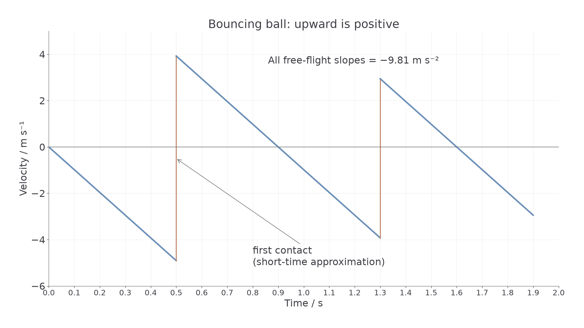
The plotted ball starts from rest and reaches $-4.905\,\mathrm{m\,s^{-1}}$ after $0.500\,\mathrm{s}$. Its initial drop is the magnitude of the triangular area, $1.226\,\mathrm{m}$. It rebounds at $+3.924\,\mathrm{m\,s^{-1}}$, reaching its next top $0.400\,\mathrm{s}$ later. The rise is $\tfrac12(0.400)(3.924)=0.785\,\mathrm{m}$, less than the original drop.

During actual contact, velocity changes continuously over a short time, giving a very steep positive gradient and a large upward acceleration; gravity still acts but the floor's force is larger. A vertical jump is an approximation to this short interval, not an infinite physical acceleration. Energy transferred to deformation, heating and sound explains the reduced rebound speed. For an acceleration–time graph, flight is a horizontal line at $-g$, while contact is a large upward pulse whose signed area gives the contact change in velocity.