RP04 - Determination of the Young Modulus
Determine the Young modulus by loading a wire, measuring small extensions and interpreting a graph. This lesson develops the measurement choices, uncertainty analysis and validity checks behind required practical 4. Written planning prepares you for practical work; performing it safely and independently requires supervised laboratory evidence.
Turn a Gradient into the Young Modulus
A tensile force on a uniform wire of original length and original cross-sectional area produces extension . In the linear elastic region,
Stress is measured in pascals and strain is dimensionless, so the Young modulus is in . The experiment must measure geometry as well as force and extension: is a wire's stiffness, which depends on its dimensions.
Rearrange into the form of a straight-line relationship:
Extension plotted against force
Here extension is vertical and force is horizontal. The gradient has units . If force is vertical instead, gradient and . Read axes before deciding which expression to use. On a stress–strain graph, the initial gradient gives directly.
Using a best-fit gradient combines information from several loads. A constant displacement zero offset changes the intercept but not the gradient; a load-dependent slip or support movement can change the gradient and therefore corrupt . A straight fitted line is not, by itself, proof that the measured displacement is all extension of the wire.
Measure Length, Diameter, Force and Extension
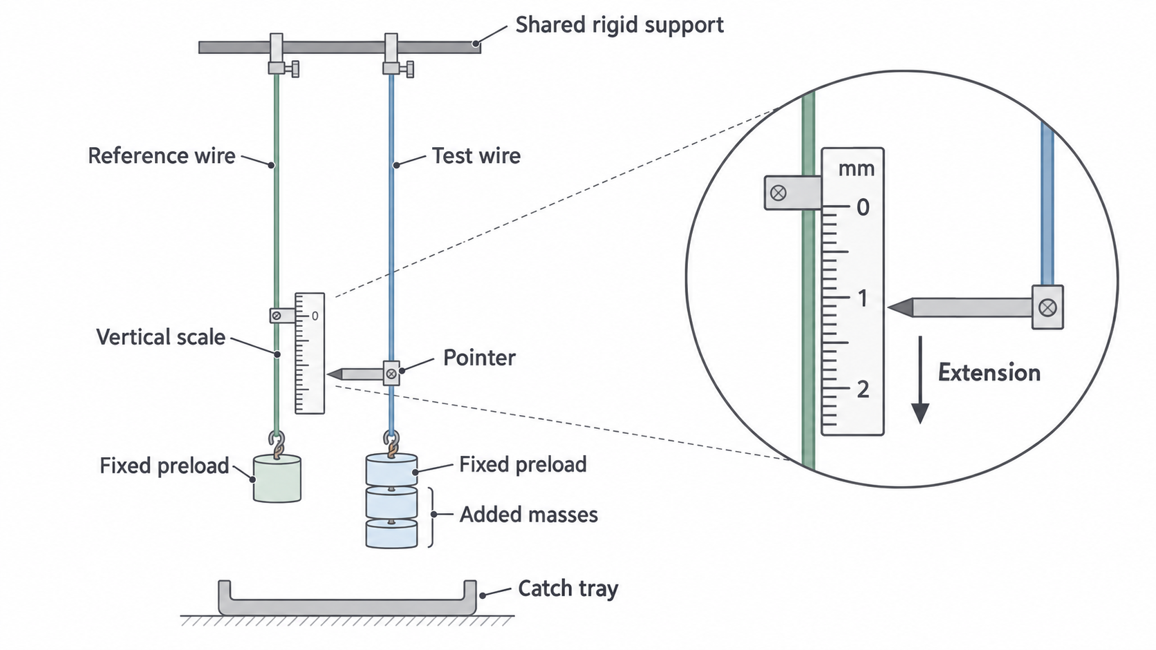
The important apparatus choice is a displacement measurement fine enough to resolve the wire's small extension. The AQA handbook describes a vertical test wire beside a reference wire, with a specialised scale and vernier reading relative vertical movement. The simplified diagram below shows that measurement principle using a pointer; it is not a diagram of the vernier's internal construction.
[DIAGRAM: asset_name: RP 04 - Determination of the Young Modulus by a Simple Method - Diagram 1; asset_slug: RP 04 - Determination of the Young Modulus by a Simple Method - Diagram 1; caption: A vertical reference scale measures the loaded test wire's downward movement; description: Two independent vertical wires share a rigid support. A vertical scale attached to the reference wire lies beside a pointer on the test wire. Fixed preloads straighten both wires and additional masses load only the test wire. Inset enlarges the scale and pointer. Catch tray below.]
Set up and record a baseline
Secure both wires using suitable clamps on a rated rigid support. Use matched wires of similar length and material for useful temperature compensation. A constant preload on each wire removes slack; the reference load stays fixed while the test load changes. Record the test wire's length from its top clamp to the pointer or vernier attachment, the section whose extension is measured. The lightly preloaded length approximates the original length because its strain is small.
Use a metre rule for this long length. A millimetre division does not mean that a two-end length measurement is known to half a millimetre: both endpoints, alignment and straightness contribute. Keep the rule parallel to the wire.
Check the micrometer's closed reading for zero error and correct subsequent diameter readings. Use the ratchet gently so the contact force is consistent. Measure diameter at several positions and in two perpendicular orientations; record all readings, the instrument resolution and any specified accuracy. A mean diameter and suit a nearly circular, uniform wire. A markedly nonuniform wire needs replacing or a more complex model, not an unexplained average.
Obtain a load series
- With the preload attached, record the displacement reading .
- Add a known mass gently to the test wire, wait for oscillations to stop, and record the new reading . Find extension . Read the scale at eye level, perpendicular to it, with the pointer close to the scale.
- Record several increasing loads and extensions across a useful range. Calculate added force : the preload is already included in the baseline. Include the hanger only if it was added after that baseline.
- Remove added masses in stages and record unloading readings at the same forces. Return to the preload and check whether the original baseline returns. Repeat suitable measurements to estimate scatter.
- Plot the accepted linear region, determine its gradient, and combine it with and . Use the measured line's intercept as a diagnostic instead of automatically forcing it through zero.
The displacement scale may read to ; a travelling microscope can resolve smaller movements. The enlarged scale in the illustration explains the geometry, not a certified numerical resolution. Choose a safe load range appropriate to the actual wire, clamps and support; a mass range used for one steel wire is not a universal instruction for every sample.
Wear goggles because a wire can recoil if it breaks. Secure the support and clamps, keep feet clear of suspended masses and position a tray to catch them. Add masses gently: an impact can cause a larger peak tension than the static load.
Choose Sensitive Measurements and Control Bias
A useful experiment makes the signal large enough to measure without leaving the region described by its equation. From , a longer wire increases extension at the same force. A thinner wire also increases extension, but increases stress and the risk of yielding or fracture. A larger extension reduces fractional uncertainty only if the absolute displacement uncertainty stays comparable.
The independent variable is added force and the dependent variable is extension. Keep the same wire, clamping points and temperature during the series so that , and material properties remain comparable. Use enough loads across the safe proportional region to distinguish a trend from scatter. Closely bunched data give an uncertain gradient even if individual readings are precise.
Why the reference wire helps
A fixed scale attached to the room would interpret downward support movement as extension. Measuring the test wire relative to the reference wire reduces movement shared by both suspension points. Similar wires at the same temperature also expand by similar amounts. These common changes largely cancel in the relative reading. Unequal support movement, unmatched lengths or temperatures, clamp slip and instrument sticking do not necessarily cancel. Inspect the apparatus and avoid nearby heaters or draughts.
A horizontal method is also valid
Clamp one end of a long wire along a bench, pass its far end over a freely rotating pulley, and suspend masses. A marker on the straight test section is read with a close scale or travelling microscope. Measure from the fixed clamp to that marker: wire beyond the marker is not part of the measured extension.
Ideally tension is . Pulley friction can make tension in the horizontal section differ from the hanging weight, and it can change on loading versus unloading. Check free motion and alignment; do not assume this error always has the same sign. Sag, slack and a slipping clamp also contribute apparent movement. A well-designed horizontal arrangement can give useful results; the method is not intrinsically invalid or always less precise.
Repeats can reduce random scatter and reveal anomalies. They do not remove a micrometer zero error, consistent parallax, an incorrectly measured or a load-dependent support shift. A digital instrument avoids scale interpolation but does not automatically remove calibration or zero errors.
Fit the Proportional Region and Check Recovery
Keep the raw displacement readings as well as calculated extensions so that a baseline or subtraction error can be traced. Put quantity and unit in each table heading; give readings to a precision justified by the apparatus. The following original illustrative dataset uses a wire of mean diameter .
| Added force / | Extension / |
|---|---|
| 4.00 | 0.43 |
| 8.00 | 0.81 |
| 12.00 | 1.25 |
| 16.00 | 1.66 |
| 20.00 | 2.08 |
| 24.00 | 2.55 |
For this example each extension has estimated uncertainty , from instrument information and repeat scatter; force uncertainty is negligible on the plotted scale. These are supplied assumptions, not universal uncertainty values for this practical.
[DIAGRAM: asset_name: RP 04 - Determination of the Young Modulus by a Simple Method - Diagram 2; asset_slug: RP 04 - Determination of the Young Modulus by a Simple Method - Diagram 2; caption: Extension–force data with a best-fit line and steepest acceptable line; description: Six points with vertical plus or minus 0.08 mm error bars. Best gradient 0.10586 mm per N and steepest permissible gradient 0.11313 mm per N. Both lines pass through all uncertainty bars.]
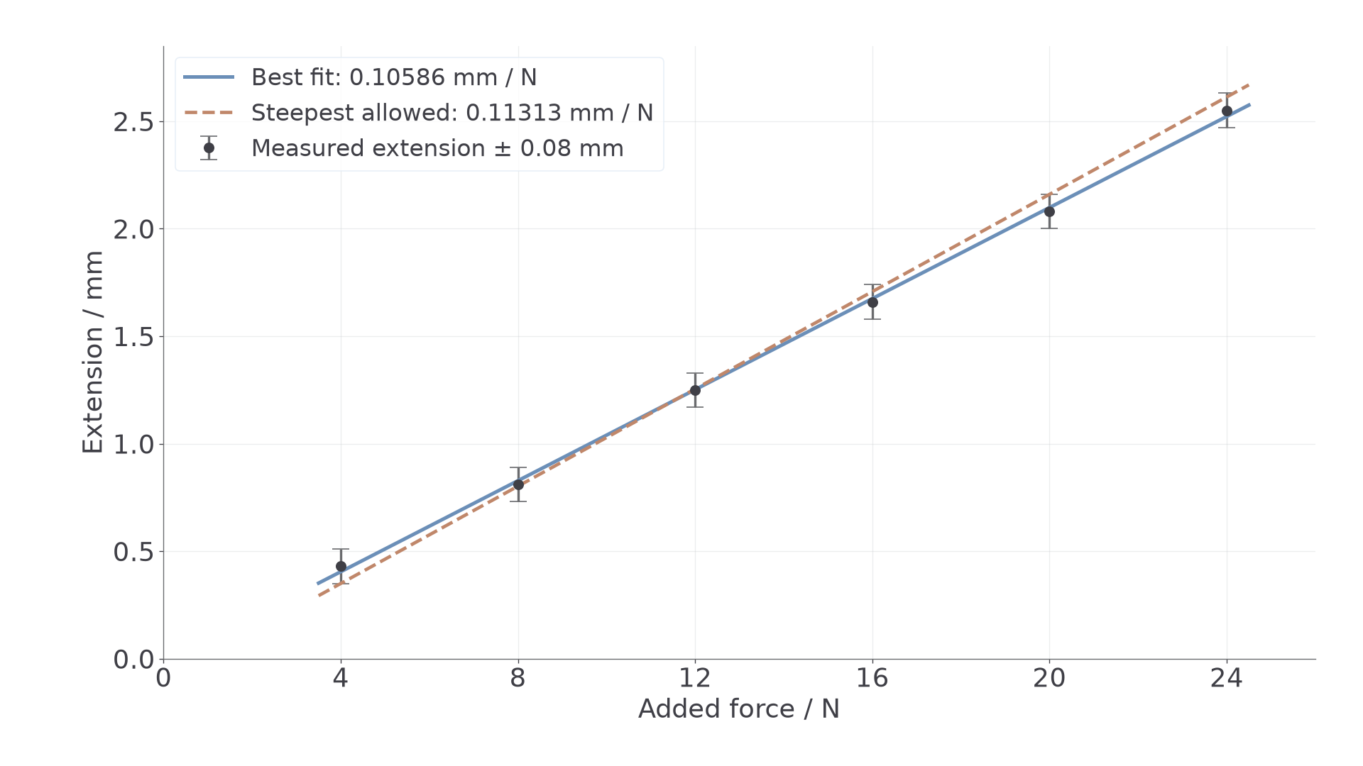
The graph is consistent with a linear relationship over this range. A fit using all six points gives and intercept . This small intercept should be assessed against measurement uncertainty; it is not evidence of a physically negative extension at zero load. Do not select only convenient points to force a preferred gradient.
What departure from the line establishes
If the increase in extension per extra force grows systematically at high load, proportionality may have ended. Check repeat readings and possible apparatus faults. Use the lower-force linear region for , with the exclusion justified by the observed trend rather than by disagreement with an expected answer.
A persistent nonzero extension after returning to the same preload supports permanent deformation, once slip and drift have been excluded. Loading and unloading readings that differ at intermediate forces may instead reflect friction, hysteresis or delayed recovery. Inspect the complete path and final baseline before deciding. Average loading/unloading results only when they agree within reasonable uncertainty and there is no systematic separation to conceal.
If the result agrees with a published modulus, it is consistent with that reference; it does not prove that every measurement was accurate, that the wire remained elastic, or that the material has been uniquely identified.
Calculate Modulus and Distinguish Graph Areas
The graph's units must be converted before using its gradient in an SI equation. For the illustrative dataset,
The best-fit gradient is . Therefore
or approximately . A gradient in millimetres used as though it were in metres would make a thousand times too small.
A systematic diameter overestimate gives an area that is too large and hence an that is too small. An extension gradient that is too large also makes too small. These directions follow from the equation, so they need not be memorised separately.
Energy requires the correct axes and starting state
For a wire loaded linearly from zero tension, is area under force vertically against extension horizontally. Dividing by original volume gives energy density , the area under a stress–strain graph. An extension–force graph has the axes reversed; do not automatically call its area the work done.
Our experiment measures extra extension from a preload. If baseline tension is and added tension is , the extra loading work is , not merely . This is why the increment graph can determine correctly without giving the total stored energy from its triangular area alone.
Propagate Uncertainty and Judge a Result
An uncertainty describes a plausible range around a measurement; it is not simply a count of displayed decimal places. Consider instrument resolution, specified accuracy, repeated spread, alignment and the actual reading procedure.
Separate readings from differences
A single scale reading may have a minimum uncertainty of half a division, but an extension found by subtracting two readings has contributions from both. Add their absolute uncertainties for a worst-case difference estimate. For example, two readings each uncertain by give an extension uncertainty of before other effects are considered.
Half the range of repeated values estimates their scatter. It does not automatically justify uncertainty smaller than the instrument's capability or eliminate calibration bias. For readings , , , , , , mean diameter is and half-range is . If that range is compatible with the instrument information, a stated estimate gives percentage uncertainty . Do not invent thousandth-millimetre individual readings from a micrometer that resolves only hundredths.
Find uncertainty in the gradient
Draw the best-fit line and steepest/shallowest lines consistent with the uncertainty bars. The worst acceptable gradient is the one furthest from the best gradient. For the example graph, steepest and shallowest are permissible; the steepest is slightly further from the best fit.
Use the AQA best-versus-worst method unless a question explicitly asks for another estimate. Half the range between extreme gradients need not equal this difference. If horizontal uncertainties matter, acceptable lines must also respect them; the vertical bars used here are a stated simplification.
Combine the contributions
For , add fractional uncertainties in products and quotients, multiplying the diameter contribution by two:
Approximate worst-case percentage uncertainty
For , and the gradient above, the contributions are , and . Total uncertainty is , giving . The gradient is the largest contribution; better displacement readings or a wider valid force range are more useful than improving the already-small length uncertainty.
If a relevant reference value is , it lies in this interval. Report consistency within estimated uncertainty, while retaining checks for systematic bias. In your laboratory report cite the reference source, material condition and temperature; keep the raw table, graph fit and uncertainty assumptions so another person can follow the conclusion. A spreadsheet may compute and display the fit, but it cannot decide which points are physically valid.