3.4.2.2 - The Young Modulus
A thick wire is harder to stretch than a thin wire of the same material. The Young modulus separates the material's stiffness from the sample's dimensions. Learn to connect stress–strain gradients, wire calculations and the measurements needed to determine this property.
Defining the Young Modulus
A material's response to a small tensile load is described by the relationship between stress and strain . In the initial proportional region, doubling the stress doubles the strain.
Young modulus
The Young modulus is tensile stress divided by tensile strain in the linear elastic region.
Material stiffness
Strain is a ratio of lengths with no unit, so has the same unit as stress: the pascal, . A large means that a given stress produces a small strain. For example, a material with under stress has strain , or .
For a particular material in the same physical condition and temperature, does not change just because a sample is longer or thicker. However, stiffness is not strength: describes the initial response, whereas breaking stress describes fracture. A high-modulus material need not withstand the largest strain or stress before breaking. At larger strains, the ratio need not remain constant, so do not use an arbitrary point on a curved graph as the Young modulus.
From Material Modulus to Wire Stiffness
A wire experiment measures force and extension directly, so substitute their definitions into the stress-to-strain ratio:
Here is original length of the measured section, is its extension, is original cross-sectional area and is tensile force. Use SI units when substituting: for a circular wire, with diameter in metres.
What changing dimensions actually changes
Rearranging gives . Comparing with gives
A uniform straight wire
This is the axial stiffness of a uniform straight wire in its linear region, not a formula for the stiffness of every coiled spring. Doubling length halves and doubles extension for the same force. Doubling diameter quadruples area and , reducing extension to one-quarter. Neither change alters itself. Keep the loading within the linear region when making such comparisons.
For example, two wires of the same material have equal lengths but one has three times the diameter. Under equal forces it has nine times the stiffness, one-ninth the stress and one-ninth the extension.
Read the Axes Before Finding a Gradient
A gradient means change in the vertical quantity divided by change in the horizontal quantity. On a graph of stress vertically against strain horizontally, the gradient of the initial straight region is the Young modulus.
[DIAGRAM: asset_name: 4.2.2 - The Young Modulus - Diagram 1; asset_slug: 4.2.2 - The Young Modulus - Diagram 1; caption: The initial stress–strain gradient gives the Young modulus; description: Stress in Pa vertically, dimensionless strain horizontally, gradient triangle entirely in the proportional region.]
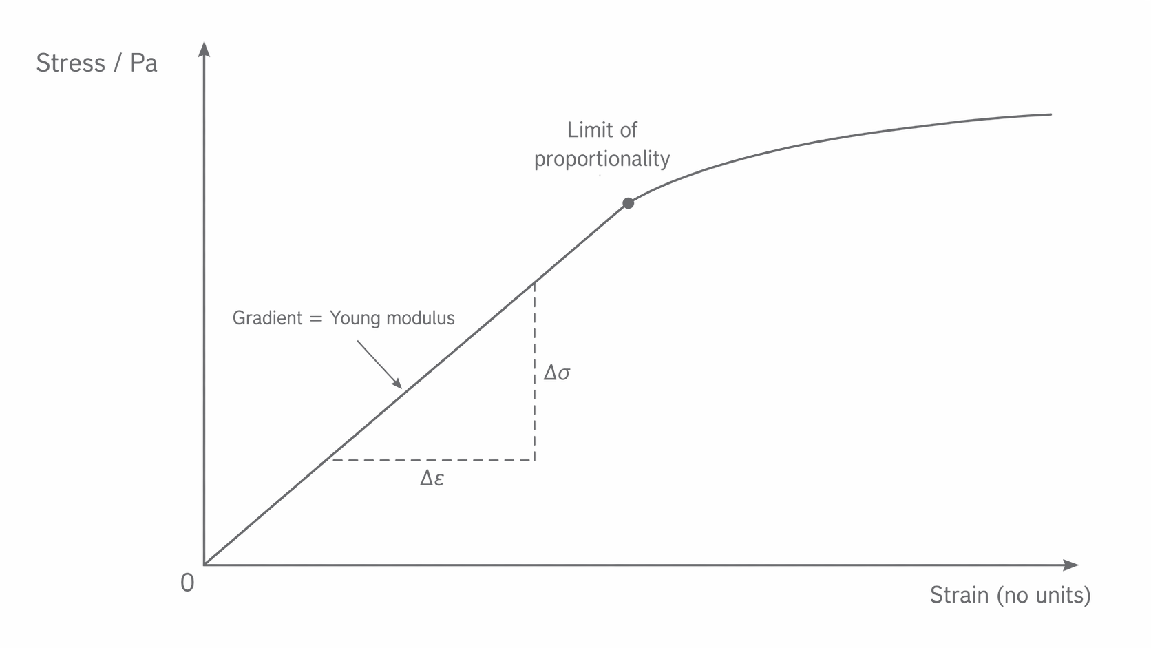
Draw a best-fit line through the appropriate data and choose widely separated points on that line. They need not be measured data points. A large gradient triangle reduces the relative effect of coordinate-reading uncertainty. Exclude the curved region from this initial-gradient determination.
Suppose line coordinates are and . Then
A strain axis labelled “strain / ” means that a coordinate of represents strain , not . Similarly .
| Vertical axis | Horizontal axis | Gradient | Recover |
|---|---|---|---|
| Stress | Strain | ||
| Force | Extension | ||
| Extension | Force |
The unit is a useful check: a force–extension gradient in is not a modulus in . A graph with strain vertically and stress horizontally would have gradient .
Measure a Wire's Force–Extension Relationship
A long, uniform wire loaded by known masses provides a simple measurement of the Young modulus. Its extension is small, so select apparatus that resolves it adequately.
[DIAGRAM: asset_name: 4.2.2 - The Young Modulus - Diagram 2; asset_slug: 4.2.2 - The Young Modulus - Diagram 2; caption: A fixed rule reads movement of a marker on a vertically loaded wire; description: Rigid top clamp, vertical wire and fixed adjacent ruler, marker near bottom, hanging masses below.]
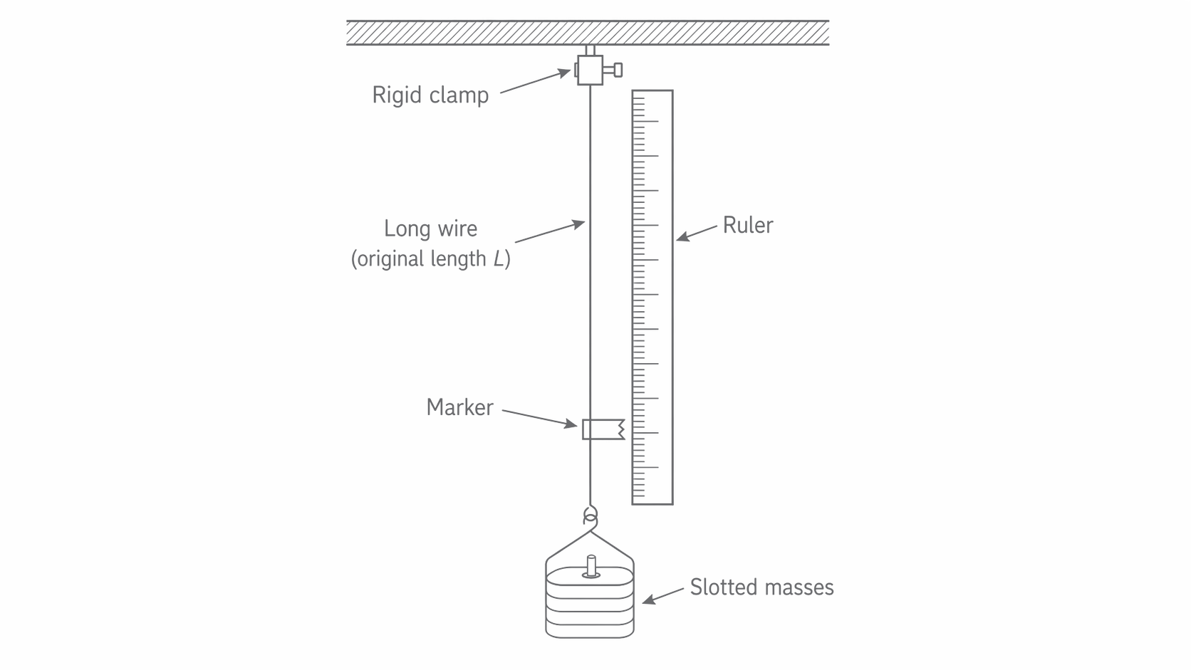
- Clamp the wire securely to a rigid support and apply a small preload to straighten it. Wear eye protection and place a catch tray below the masses. Choose loads suitable for the wire and support.
- Measure length from the top clamp to the marker, the section whose extension will be measured. This nearly unstretched, lightly preloaded length is a practical approximation to original length.
- Check a micrometer for zero error. Use its ratchet gently to measure diameter at several positions and two orientations. A mean diameter is reasonable for a nearly uniform circular wire; substantial variation means the simple uniform-area model is poor.
- Place a scale close and parallel to the marker's movement. Record its baseline reading with the preload attached. Add masses gently, wait for settling, and subtract the baseline reading from each new reading. Read perpendicular to the scale to limit parallax. If a millimetre rule cannot resolve the extension adequately, use a vernier displacement scale or travelling microscope.
- Use the added mass to find added force because extension was measured relative to the preload. Collect a useful range of loads within the linear region. Unload and check for a persistent change from the baseline; also compare repeated readings at the same load.
- Plot force against extension, fit the linear region and find . Then calculate , with .
A longer wire gives a larger extension at the same stress, reducing fractional extension uncertainty. Increasing load can help too, but eventually invalidates the proportional model or breaks the wire. A rigid support reduces spurious marker motion; a matched reference wire can compensate for common support movement and temperature change, as developed in RP04.
A return to baseline supports elastic behaviour. A straight loading graph supports proportional behaviour. Check both: neither observation alone establishes the other. Do not average visibly separated loading and unloading paths to hide a problem.
Measure diameter with calipers
For a thicker rod or cable, calipers may resolve its diameter adequately. For a thin wire, a micrometer usually gives a smaller fractional diameter uncertainty. Choose using the instrument's range, resolution and specified accuracy, not just its name.
Clean the measuring faces and close the jaws gently to check zero. Record a signed zero error, or reset a digital instrument with the clean jaws closed. Use the large external jaws for an outside diameter; the smaller internal jaws measure an inside width. Place the rod squarely between opposite measuring faces, with the measuring direction perpendicular to its length. Avoid tilted jaws or excessive pressure. Repeat at several positions and orientations to check uniformity.
A vernier scale resolves fractions of a main-scale division. Read it perpendicular to the scales:
- Read the main-scale graduation immediately before the vernier zero.
- Find the vernier graduation that coincides with a main-scale graduation. Count its divisions from the vernier zero and multiply by the stated vernier resolution.
- Add this fraction to the main-scale reading, then subtract the signed zero error.
For example, if ten vernier divisions span nine main-scale divisions, one vernier division is . The difference, , is this instrument's resolution. A main-scale reading of and coincidence at the sixth vernier division give . If the closed jaws read , the corrected diameter is . Other vernier scales have different resolutions: check the scale provided.
A digital caliper gives the reading directly. A display that changes in steps has resolution ; this does not establish an uncertainty of . Instrument accuracy, jaw alignment, zero error and repeated-reading spread also matter.
Calculate Tension and Stored Energy
The same wire geometry links extension to force and then to stored energy. Keep intermediate values unrounded and check that the question permits the linear model.
A uniform steel wire has diameter , original length and extension under linear elastic loading. Its modulus is .
First convert diameter and extension to metres:
Then the tension is
For negligible dissipation and loading from zero force, the force–extension area gives
Combining the expressions gives . Dividing by original volume gives : area under a stress–strain graph is energy per unit volume, not the total energy. For example, in a sample corresponds to .