3.7.2.4 - Orbits of Planets and Satellites

Circular-orbit speed, period and graph tests

A circular orbit needs an inward acceleration even when speed is constant, because velocity changes direction. In the model below gravity alone supplies that acceleration: a satellite of mass $m$ orbits a much larger spherical mass $M$, with negligible drag, thrust and influence from other bodies. Measure orbital radius $r$ from the source centre.

Equate gravitational force to the required centripetal force, rather than adding “centripetal force” as a second physical interaction:

The satellite mass cancels. For the same source, a higher circular orbit has lower speed. Doubling radius reduces speed by $1/\sqrt2$. The force is radial and velocity tangential, so gravity changes velocity’s direction without doing work in this circular orbit.

For one circuit, $v=2\pi r/T$. Substituting into the force relation gives

Thus $T^2\propto r^3$ for circular orbits around the same central mass. If the radius doubles, the period becomes $2^{3/2}=2\sqrt2$ times as long. An elliptical orbit has changing speed and radius; the constant-radius derivation must not be applied to its instantaneous radius.

Inferring a central mass and testing a power law

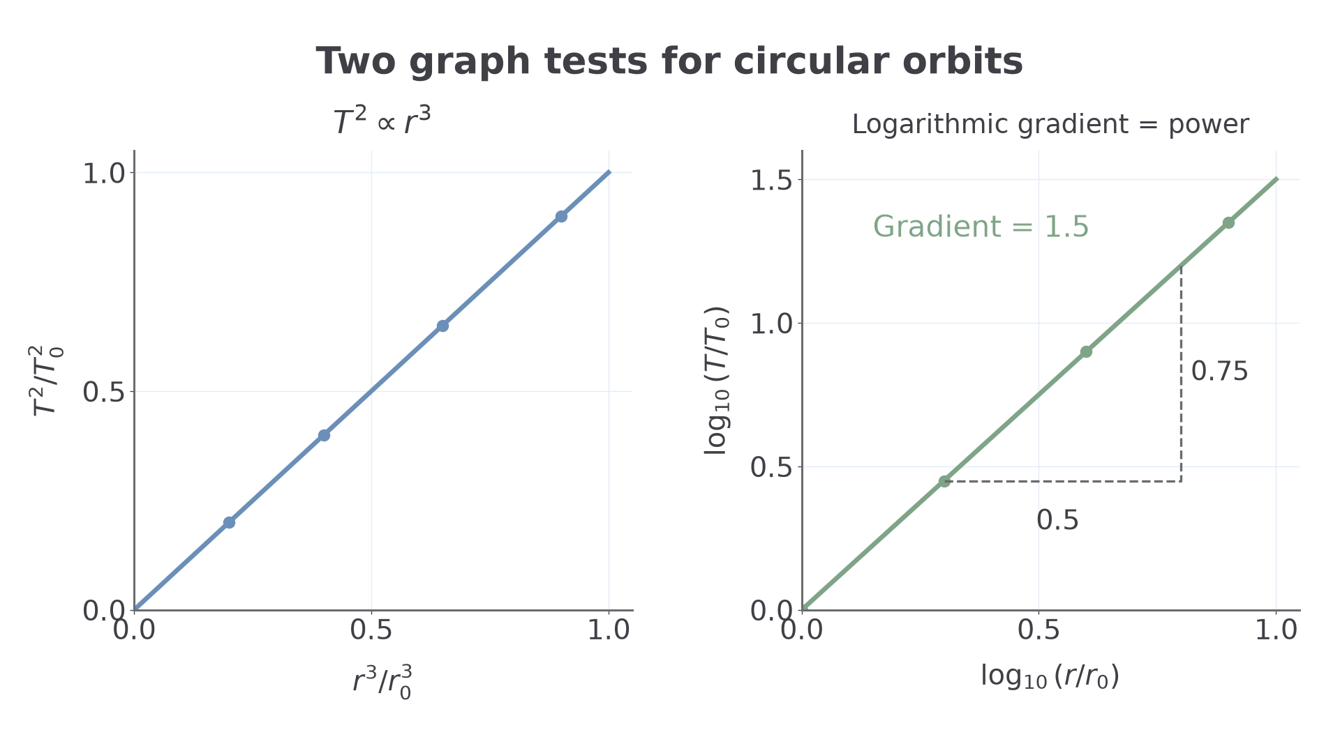
A plot of $T^2$ against $r^3$ is a straight line through the origin, with gradient $4\pi^2/(GM)$ in $\mathrm{s^2\,m^{-3}}$. Rearrange the gradient to infer $M$. For example, a gradient $9.86\times10^{-14}\,\mathrm{s^2\,m^{-3}}$ gives $M=6.00\times10^{24}\,\mathrm{kg}$ using $G=6.67\times10^{-11}\,\mathrm{N\,m^2\,kg^{-2}}$.

Choose a reference radius $r_0$ and let $T_0$ be its circular-orbit period around the same mass. Taking logarithms gives

The reference values make the ratios dimensionless. A plot of $\log(T/T_0)$ against $\log(r/r_0)$ has gradient $1.5$, not $3$. A plot of $\log(T^2/T_0^2)$ against $\log(r/r_0)$ instead has gradient $3$. Read both axes before interpreting a logarithmic gradient.

[DIAGRAM: asset_name: 7.2.4 - Orbits of Planets and Satellites - Diagram 1; asset_slug: 7.2.4 - Orbits of Planets and Satellites - Diagram 1; recommended_method: retained_png; caption: Circular-orbit graph tests. T₀ is the period at radius r₀. The logarithmic gradient is 1.5.; description: Exact circular-orbit plots for one central mass: T² against r³ is linear, while log(T/T₀) against log(r/r₀) has gradient 1.5. The points are model satellite data, not evenly spaced real planets.]

For an order-of-magnitude check on Earth’s orbital kinetic energy, estimate $M_S\sim2\times10^{30}\,\mathrm{kg}$, $m_E\sim6\times10^{24}\,\mathrm{kg}$ and $r\sim1.5\times10^{11}\,\mathrm m$. Then $v\sim3\times10^4\,\mathrm{m\,s^{-1}}$ and $K\sim\tfrac12(6\times10^{24})(3\times10^4)^2\sim3\times10^{33}\,\mathrm J$.

Kinetic, potential and total orbital energy

A circularly orbiting satellite has positive kinetic energy and negative gravitational potential energy when the zero is at infinity. Substituting $v^2=GM/r$ gives

Thus $U=-2K$ and $E=-K=U/2$ for a circular orbit. The negative total energy means the satellite is gravitationally bound in this isolated two-body model. Potential energy being negative alone is insufficient: a sufficiently fast object can have nonnegative total energy and escape.

[DIAGRAM: asset_name: 7.2.4 - Orbits of Planets and Satellites - Diagram 2; asset_slug: 7.2.4 - Orbits of Planets and Satellites - Diagram 2; recommended_method: retained_png; caption: Energies of alternative circular orbits: U = −2K and E = −K. R and E₀ are fixed reference scales.; description: Exact circular-orbit energies. The fixed reference E₀ = GMm/(2R) makes the vertical coordinate dimensionless; at each radius U = −2K and E = −K. These are alternative circular orbits, not successive positions in one ellipse.]

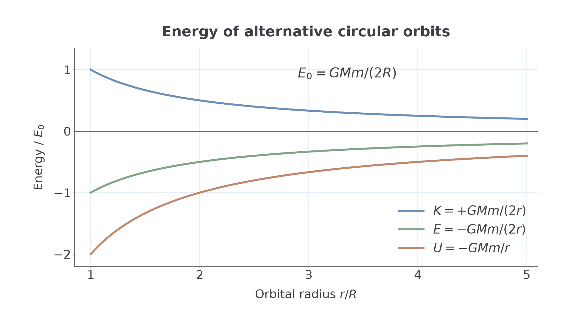
Compare two circular orbits. At larger $r$, $K$ decreases, $U$ increases towards zero, and $E$ increases towards zero. Energy must therefore be supplied to reach the higher circular orbit even though the final speed is lower. The potential-energy increase is twice the magnitude of the kinetic-energy decrease.

For a $400\,\mathrm{kg}$ satellite raised from $r_1=7.0\times10^6$ to $r_2=8.0\times10^6\,\mathrm m$ around $M=6.0\times10^{24}\,\mathrm{kg}$,

The final kinetic energy is lower by $1.43\times10^9\,\mathrm J$, while potential energy rises by $2.86\times10^9\,\mathrm J$. A real transfer involves thrust and a non-circular path between these two states; the circular formulas describe its endpoints. Conversely, slow orbital decay through weak drag can reduce total energy while the speed of the eventual lower orbit is higher.

Escape speed from energy conservation

Escape speed is the minimum initial speed at a specified radius that lets an unpowered object reach indefinitely large distance with no remaining kinetic energy. The often-used name “escape velocity” refers to this speed threshold, not a single required direction.

Assume an isolated, non-rotating spherical source, no atmosphere or other dissipative force, no further thrust and a trajectory that does not hit the source. Energy conservation for marginal escape gives