3.13.5.3 - Astables
Interpret clock pulses by their period, frequency, pulse width and duty cycle, and explain how an external resistor–capacitor network controls an astable’s running frequency.
An oscillator supplies clock edges
An astable is an oscillator with no stable output state: while powered and enabled, it repeatedly switches between high and low without a separate trigger for every pulse. Its output can provide the clock for a counter.
A counter triggered by rising edges advances once per complete astable cycle. It does not keep counting throughout the high level, and its falling edge is not a second count. An ideal 100 Hz pulse train gives 100 active rising edges each second, provided the counter is enabled and the pulse widths satisfy the device's requirements.
[DIAGRAM: asset_name: E.5.3 - Astables - Diagram 1; asset_slug: E.5.3 - Astables - Diagram 1; caption: The high and low intervals together form one complete period; description: The high and low intervals together form one complete period]
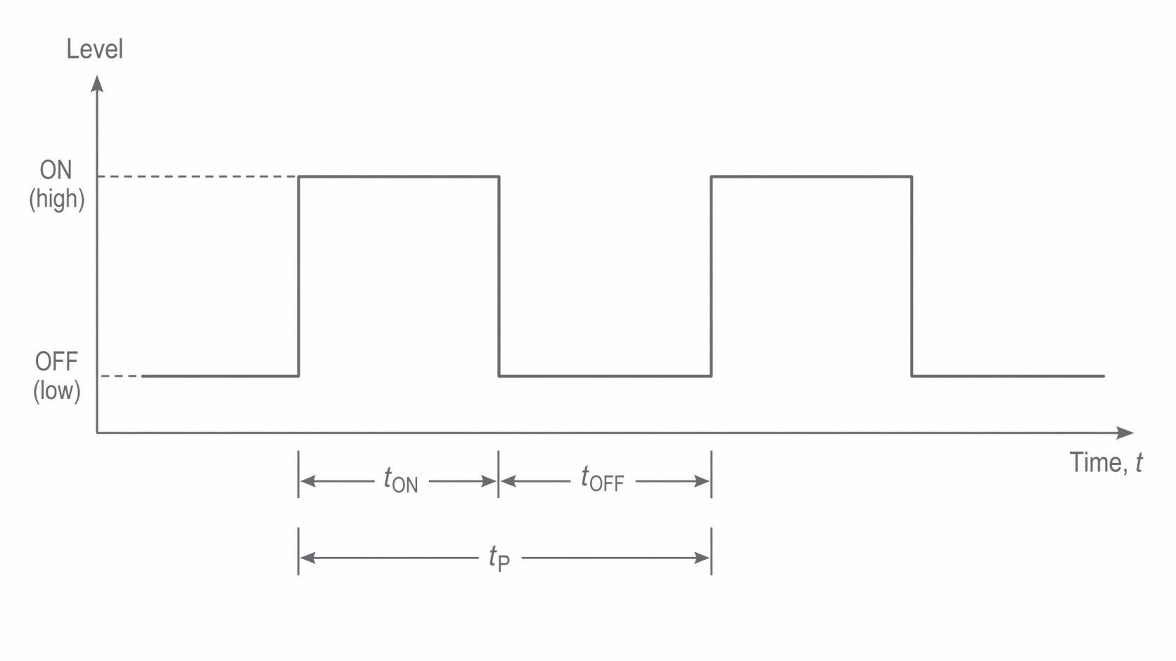
The period, written T or , runs between corresponding points on consecutive cycles, such as rising edge to rising edge. The high interval is the mark or ON time; the low interval is the space or OFF time. A rectangular waveform can have unequal intervals. “Square wave” is often used for the special case with equal high and low times.
Real transitions take a finite time. Ideal rectangular plots make the timing relationships clear; when interpreting an actual trace, use a consistent level to identify corresponding edges. A change in pulse height alone does not determine a change in frequency.
Measuring pulse timing
The duration of the high and low intervals determines both how often pulses recur and how much of each cycle is high. Keep the denominators distinct when calculating duty cycle and mark-to-space ratio.
| Quantity | Meaning and relationship |
|---|---|
| Period T | Time per full cycle: |
| Frequency f | Cycles per second: , in Hz |
| Pulse width | High time for these positive pulses |
| Duty cycle | , or |
| Mark-to-space ratio |
From times to waveform quantities
If high time is 3.0 ms and low time is 2.0 ms, . Convert to seconds before taking the reciprocal:
The duty cycle is , and the mark-to-space ratio is 3:2. The ratio is not 60%: it uses the low time, rather than the whole cycle, as the comparison.
Conversely, at 250 Hz the period is 4.0 ms. A 3:1 mark-to-space ratio splits this into four equal parts, giving 3.0 ms high and 1.0 ms low. In general a ratio m:s gives duty cycle . A 50% duty cycle gives 1:1, but it does not specify the frequency.
Reading an oscilloscope trace
Multiply horizontal divisions by the time-base setting to obtain a time. If one complete cycle spans 4.0 divisions at , its period is 2.0 ms and its frequency is 500 Hz. Measure between two corresponding rising edges, not from a rising edge to the next falling edge. Measuring several complete cycles and dividing by their number reduces the fractional effect of reading each endpoint; it does not remove time-base calibration error.
Continue this lesson.
You’re previewing NovaLearn without an account. Create a free account to read the rest.
Create free account