3.11.1.3 - Rotational Motion
Use angular displacement, velocity and acceleration to describe rotation. Graphs reveal how the motion changes, while constant-acceleration equations connect speeds, times and angles, including stopping and reversal.
Angular quantities and direction
Angular displacement is the change in angular position about a chosen axis. Choose one sense of rotation as positive and keep that convention throughout a calculation.
One revolution is . Since one revolution is , convert degrees using . For example, ; in reverse, multiply a radian value by to obtain degrees. The angular speed is how fast the object turns, without a direction. Angular velocity includes its rotational sense; for a fixed axis we represent that sense by a sign. Speed is the magnitude of angular velocity, so it cannot be negative.
Over a time interval, the average angular velocity and average angular acceleration are
Their units are and . At an instant these quantities are local rates of change, found from tangents to the relevant graphs. For a constant rate, the interval formula gives the rate throughout that interval. For a varying rate, a sufficiently short interval approximates the instantaneous value.
Negative acceleration does not always mean slowing down. If and , the object turns faster in the negative sense. It slows when angular velocity and acceleration have opposite signs.
Connecting linear and angular motion
Linear and angular variables have matching mathematical roles, but they measure different features of motion.
| Linear quantity | Angular counterpart |
|---|---|
| Displacement | Angular displacement |
| Initial and final velocity | |
| Acceleration | Angular acceleration |
| Time | The same time |
For a point at fixed radius , arc length is , tangential speed is , and tangential acceleration is . These relations use radians. A rigid wheel shares one and one , but points farther from the axis travel faster and have greater tangential acceleration.
Tangential acceleration changes the speed. The radial acceleration changes the direction of motion and exists even when . Do not confuse a centrifuge's large radial acceleration at steady speed with its angular acceleration during spin-up.
To convert , first divide by 60 to get , then multiply by : . Carry exact values or extra digits through intermediate work.
Reading gradients and areas
The gradient and area of an angular-velocity–time graph describe different physical quantities.
The gradient is angular acceleration. A straight line has constant gradient and hence uniform angular acceleration; a curve needs a tangent to find at a chosen instant. The signed area between the graph and time axis is angular displacement. Areas below the time axis count negatively; add their magnitudes instead when finding total angle travelled.
[DIAGRAM: asset_name: C.1.3 - Rotational Motion - Diagram 1; asset_slug: C.1.3 - Rotational Motion - Diagram 1; caption: Angular-velocity graphs with an exact gradient triangle and a tangent for changing acceleration; description: Angular-velocity graphs with an exact gradient triangle and a tangent for changing acceleration.]
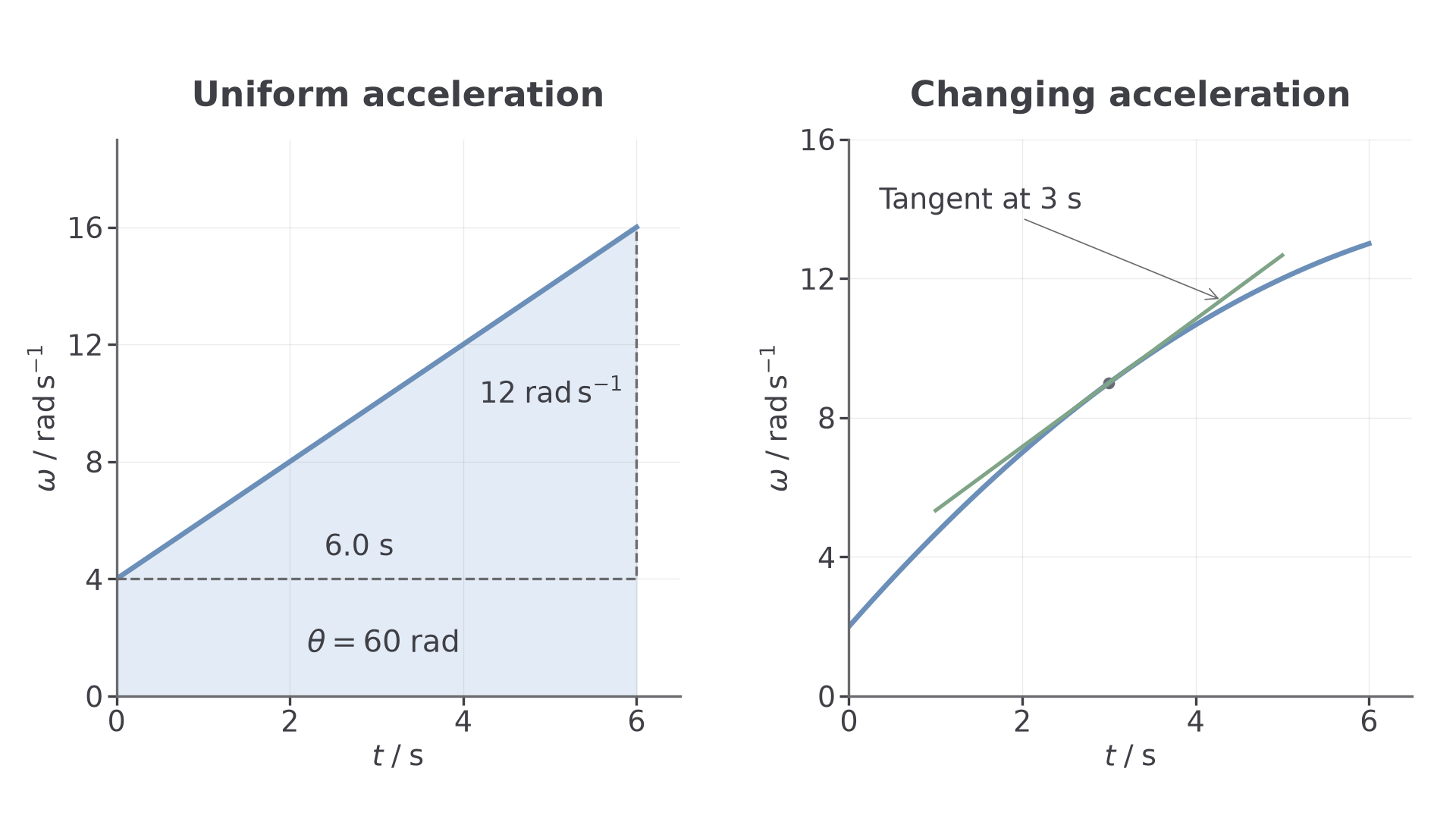
For the straight line shown, . Its displacement is the trapezium area . The area contains both the rectangle from the initial velocity and the triangle due to acceleration.
For the curved graph, a chord between distant points gives an average acceleration. Use the tangent for the instantaneous value. For measured data with varying acceleration, sum trapezium areas between successive readings to estimate displacement; shorter intervals can improve the estimate if the measurements remain reliable.
A displacement–time graph works differently: its gradient is angular velocity, not acceleration.
Continue this lesson.
You’re previewing NovaLearn without an account. Create a free account to read the rest.
Create free account