3.13.4.4 - Real Operational Amplifiers
Real op-amps have finite gain, loading effects and a limited frequency response. Read logarithmic response curves, calculate the gain–bandwidth trade-off, and use output-range and bandwidth requirements together when judging a design.
Limits of the Ideal Model
A real op-amp approximates the ideal model over a useful operating range. Its limitations depend on the device, supply, temperature, load and frequency; there is no single set of numerical values shared by all op-amps.
| Ideal assumption | Real behaviour and consequence |
|---|---|
| Infinite open-loop gain | Finite gain means a small non-zero input difference is needed for a given output. |
| Infinite input resistance | Finite input resistance and input bias currents can load a high-resistance source. |
| Zero output resistance | Non-zero output resistance can cause a voltage drop when load current is drawn. Feedback reduces the effective output resistance. |
| Unlimited frequency response | Gain falls at high frequency, limiting useful bandwidth. |
| No input offset | A small input-referred offset can create an unwanted output even with equal intended inputs. |
For illustration, needs an input difference of for a output. Treating the input voltages as equal can therefore be an excellent approximation without being exact.
Input offset voltage is the small differential voltage that would have to be applied to make the output zero under specified conditions. It is not simply the resulting output error. With very large open-loop gain, a tiny offset may even drive an open-loop output to saturation. Some devices provide offset adjustment; do not assume every op-amp has offset-null pins.
Real output swing is constrained by the power rails and may fall noticeably short of them. Rail-to-rail devices approach the rails more closely, with limits still dependent on load. Output current is limited separately: non-zero output resistance and maximum safe output current are related practical concerns, not identical definitions.
Reading Frequency Response
A frequency response plots gain magnitude against signal frequency. Logarithmic frequency scales fit a wide range on one graph: equal distances represent equal ratios, not equal additions. On a log scale the midpoint between and is , not .
[DIAGRAM: asset_name: E.4.4 - Real Operational Amplifiers - Diagram 1; asset_slug: E.4.4 - Real Operational Amplifiers - Diagram 1; caption: Open-loop response: the smooth curve and straight-line approximation share a 10 Hz corner and 10 MHz unity-gain frequency; description: Open-loop response: the smooth curve and straight-line approximation share a 10 Hz corner and 10 MHz unity-gain frequency.]
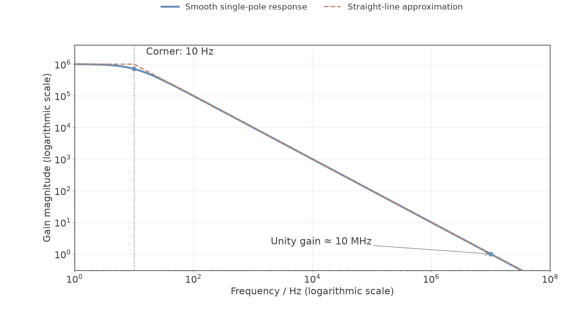
The low-frequency open-loop gain in this example is . At higher frequency the gain rolls off. The dashed straight-line approximation has a horizontal plateau and a descending line whose intersection identifies the break or corner frequency, . In the descending region a tenfold increase in frequency gives approximately a tenfold decrease in gain.
A real transition is rounded, not an abrupt change. For the single-pole model shown, gain at the corner is about of the low-frequency gain: a reduction. The usual bandwidth of a response extending from dc is the frequency from zero to this upper cutoff. Being inside the bandwidth does not mean the gain is exactly constant right up to the edge.
The horizontal logarithmic axis cannot show zero, but that does not mean the amplifier excludes dc. The vertical scale here shows linear gain magnitude on a logarithmic axis. If a graph instead uses gain in decibels, unity gain is , and is plotted on an ordinary dB scale; do not multiply dB values by frequency.
The Gain–Bandwidth Trade-Off
Negative feedback gives a lower, more predictable low-frequency gain and a larger bandwidth. For the standard approximately single-pole op-amp model used in AQA calculations,
where is the positive gain magnitude, is bandwidth in hertz and is the gain–bandwidth product in hertz. Do not use a negative signed gain to obtain a negative bandwidth. At unity gain, the bandwidth is approximately .
For and non-inverting gain , . Reducing the gain to increases the bandwidth to . Requiring bandwidth at least therefore places an upper bound in this model.
Continue this lesson.
You’re previewing NovaLearn without an account. Create a free account to read the rest.
Create free account