3.1.2 - Limitation of Physical Measurements
A measurement is an estimate supported by evidence, not an exact truth. Learn to diagnose errors, assign realistic uncertainties, carry them through calculations and graphs, and decide which experimental improvement will matter most.
Random and systematic errors
An error is the difference between a measured value and the true value. Usually the true value is unknown, so the exact error is unknown too. An uncertainty describes the doubt in a result; it is not a correction you automatically add to the reading.
Random errors vary unpredictably between readings and produce scatter. Variation in reaction time and electrical noise are examples. Independent repeat measurements and a mean usually reduce the effect of random variation on the final estimate. They do not make the spread of individual readings disappear or guarantee that the mean is correct.
Systematic errors produce a consistent bias: for example, a balance with a positive zero offset makes every mass too large. The bias need not always be a fixed amount; a calibration error can be proportional to the reading. Repeating and averaging preserve that bias. Check a known reference, correct an observed zero offset or change the flawed method.
Reading a scale from the same wrong angle can cause a systematic parallax error. If the viewing angle varies, it can also contribute scatter. Classify the error by its effect, not just by the name of the apparatus.
[DIAGRAM: asset_name: 1.2 - Limitation of Physical Measurements - Diagram 1; asset_slug: 1.2 - Limitation of Physical Measurements - Diagram 1; recommended_method: retained_png; caption: Repeats can cluster away from the true value or scatter around it.; description: A tight cluster displaced from the true value compared with a wider cluster centred approximately on it.]
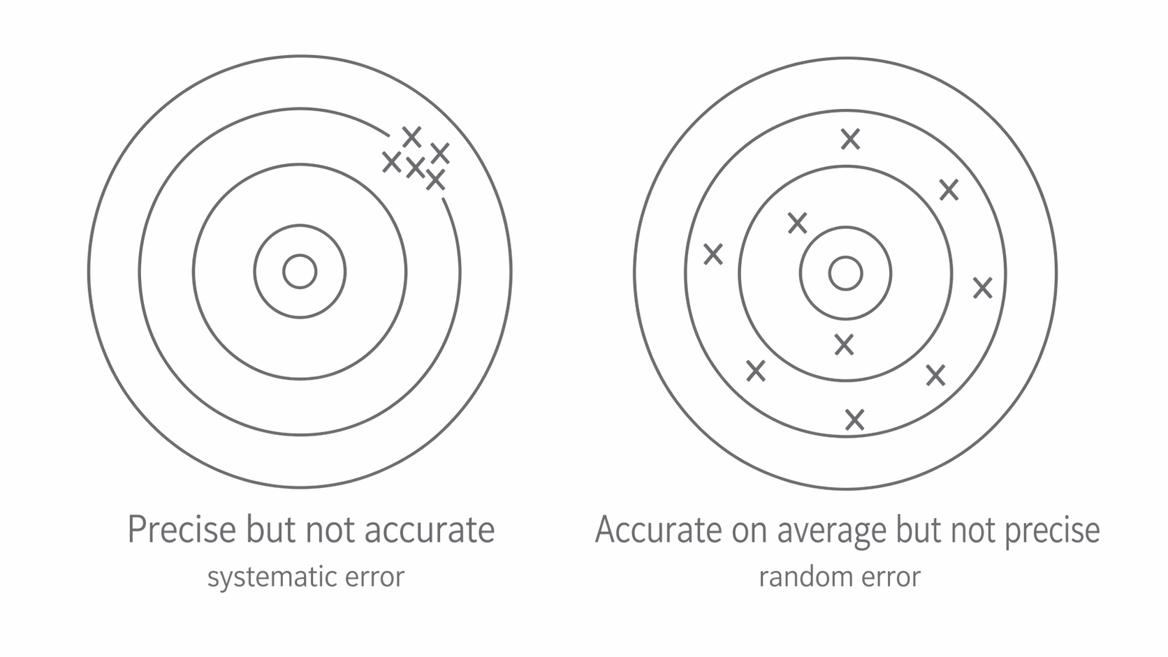
The target centre represents the true value. The left cluster has little scatter but is biased. The right cluster has more scatter and a mean near the centre. Real experiments can contain both kinds of error, so low scatter alone does not establish accuracy.
Investigate an anomalous reading rather than quietly discarding an inconvenient value. Recheck the measurement and method; exclude a reading only with a reason. If a question states that all repeats are valid, use all of them.
Describing measurement quality
Measurement quality has several different aspects: agreement among repeats, agreement with the true value, and the ability of the instrument to distinguish small changes.
| Term | What it describes |
|---|---|
| Precision | Little spread among repeated measured values. |
| Repeatability | Consistent results when the same person uses the same method and equipment under the same conditions. |
| Reproducibility | Consistent results when the person, equipment or method changes. |
| Resolution | The smallest change in the measured quantity that produces a detectable change in the reading. |
| Accuracy | Closeness of a result to the true value. |
“Consistent” means agreement within the relevant uncertainty, not necessarily identical calculator digits. A millimetre ruler has a resolution of . A digital stopwatch may display steps of , but human start/stop judgement may be uncertain by much more than that. More displayed digits do not remove the observer's reaction-time uncertainty.
A precise set can be inaccurate because of systematic error. Random error can also make an individual reading inaccurate: accuracy is not a synonym for “absence of systematic error”. Reproducibility adds useful evidence, but two instruments sharing the same calibration bias could still agree with each other.
Estimating and reporting uncertainty
Write a result as , where is the absolute uncertainty, in the same unit as . For example, gives an estimated interval from to . It is a statement of reasonable doubt, not a guarantee that the true value is inside.
Here the fraction is , or . Fractional uncertainty has no unit. A percentage uncertainty is not useful for a value of zero; report an absolute uncertainty instead.
Choose the uncertainty from the method
- For a single judgement on an analogue scale, half the smallest division is a common minimum estimate, assuming the scale can be read clearly. A division gives for one position.
- If a length is found by judging two positions, each contributes uncertainty. With at each end, the length has . Poor alignment or an indistinct edge can make it larger.
- For a digital instrument, use the quoted manufacturer's uncertainty or the question's stated convention. Resolution alone is not its complete uncertainty. AQA's practical guidance allows half a final-digit step as a starting estimate if nothing else is given, normally rounded up to one step when reporting value and uncertainty together. For a display stepping by , a commonly reported resolution-based estimate is therefore .
- For repeated valid readings, the half-range, , is the usual A-level estimate of the scatter uncertainty. Do not quote zero uncertainty merely because repeats round to the same displayed value; instrument and method limits remain.
For valid times , and , the mean is and half-range is . This supports , rather than choosing the stopwatch's smaller display step and ignoring the observed scatter.
Timing many cycles and reporting digits
If an exactly counted cycles take , the period is and . Timing more cycles reduces the percentage uncertainty if the absolute start/stop uncertainty stays approximately the same. Repeating whole runs is separately useful for estimating scatter and detecting anomalies.
Record instrument readings at their displayed resolution and retain extra digits during calculations. For a final result with stated uncertainty, usually give the uncertainty to one or two significant figures and round the value to the same decimal place: a calculated with uncertainty becomes . Without an explicit uncertainty, use the precision of the supplied data to choose sensible significant figures. Follow a specifically requested precision.
Combining uncertainties in calculations
The uncertainty of a calculated quantity depends on how its measured inputs enter the equation. The following A-level rules estimate a maximum uncertainty; they are not a statistical confidence calculation. For products and powers they are small-uncertainty approximations.
Sums and differences: add absolute uncertainties
For or , use . Subtracting two readings does not subtract their possible uncertainties: one reading could be high while the other is low.
For independent scale readings and , the difference is . Its percentage uncertainty is about , large because the measured difference is small. A known common additive zero offset would cancel in a difference; do not count the same shared offset twice as if it were independent reading scatter. Use the uncertainty model supplied in the question.
Products and quotients: add fractional or percentage uncertainties
For or ,
For and , . The percentage contributions are and , giving . The absolute uncertainty is , so report .
Powers: multiply by the magnitude of the power
For ,
Squaring a radius doubles its percentage uncertainty; taking a square root halves it; an inverse square still doubles it, since uncertainty is positive. Exact numerical factors such as 2 and contribute no uncertainty.
For , . Radius uncertainty is , so area uncertainty is , or . A consistent rounded result is .
For a more complicated expression, identify each power before adding contributions. If , then
Error bars, gradients and intercepts
An error bar extends from a measured point to the limits set by its uncertainty. A vertical bar for has total length ; horizontal bars show uncertainty in . They describe the data, not the uncertainty in the fitted line itself.
[DIAGRAM: asset_name: 1.2 - Limitation of Physical Measurements - Diagram 2; asset_slug: 1.2 - Limitation of Physical Measurements - Diagram 2; recommended_method: matplotlib; caption: Each vertical bar extends 0.20 V above and below its measured point.; description: Voltage measurements against current, each with a vertical uncertainty of 0.20 V; the line follows the trend without passing through every central point.]
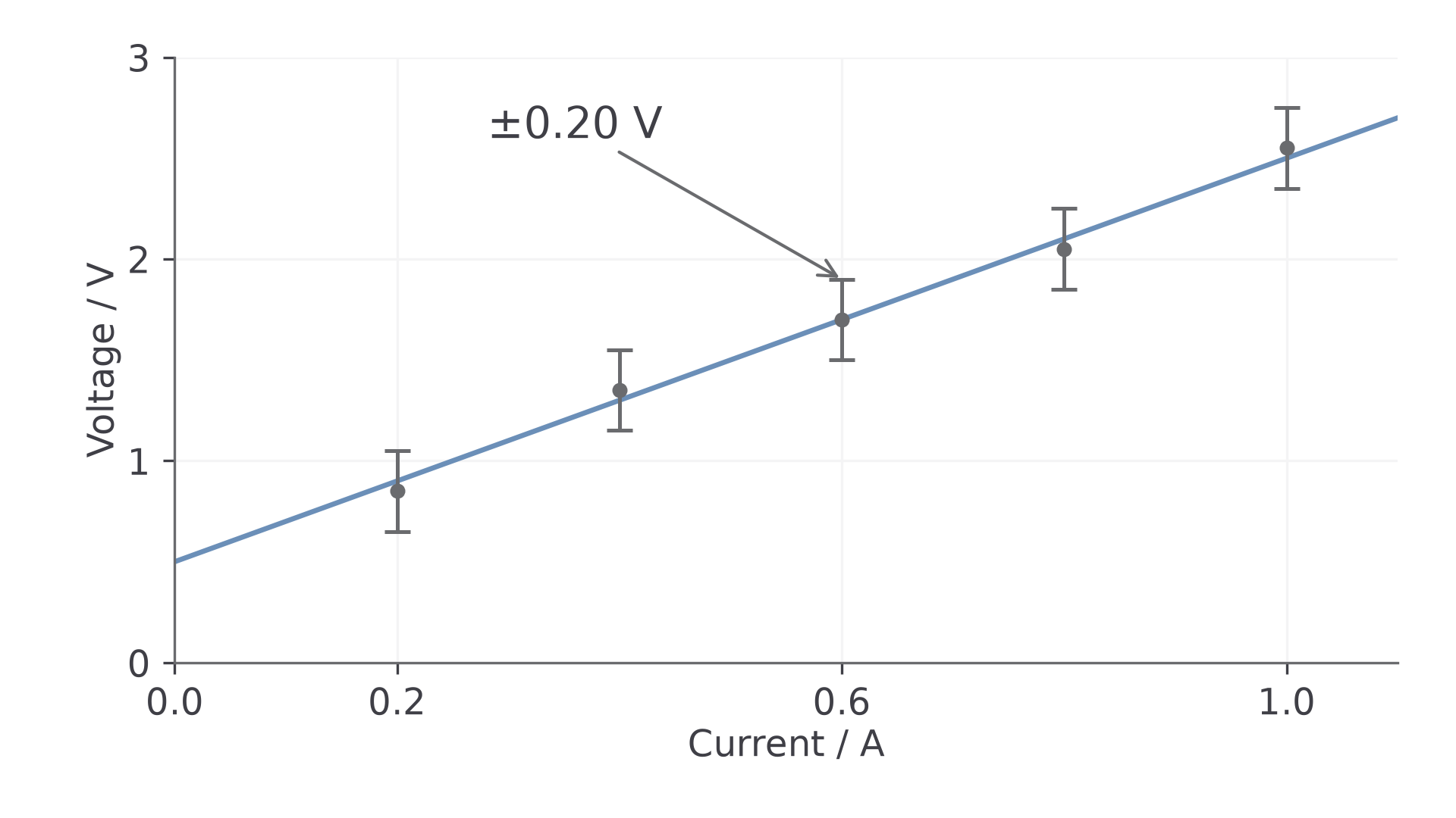
Choose a best-fit line representing the trend, with points reasonably balanced on either side. Do not join successive points or force the line through the origin unless the model and evidence justify it. If a straight line cannot fit the uncertainty ranges, investigate the model, underestimated uncertainties or anomalies; do not discard points simply to make it fit.
Gradient and intercept uncertainty
Draw the steepest and shallowest acceptable lines consistent with the uncertainty bars. Check all the bars: a line through opposite ends of the first and last bars can still miss an intermediate one. With uncertainty in both axes, check the corresponding uncertainty rectangles. If bars are absent, estimate extreme lines reasonably consistent with the scatter; their choice is less tightly constrained and should be justified.
For each line use two well-separated points on that line, not necessarily measured points, to calculate . Read the intercept where the line reaches ; it is not the value at the left edge if that edge is at non-zero .
[DIAGRAM: asset_name: 1.2 - Limitation of Physical Measurements - Diagram 3; asset_slug: 1.2 - Limitation of Physical Measurements - Diagram 3; recommended_method: matplotlib; caption: Acceptable extreme lines cross every error bar. Each bar shows ±0.10 V.; description: Best, steepest and shallowest lines pass through every voltage error bar; their different gradients and voltage intercepts are shown.]
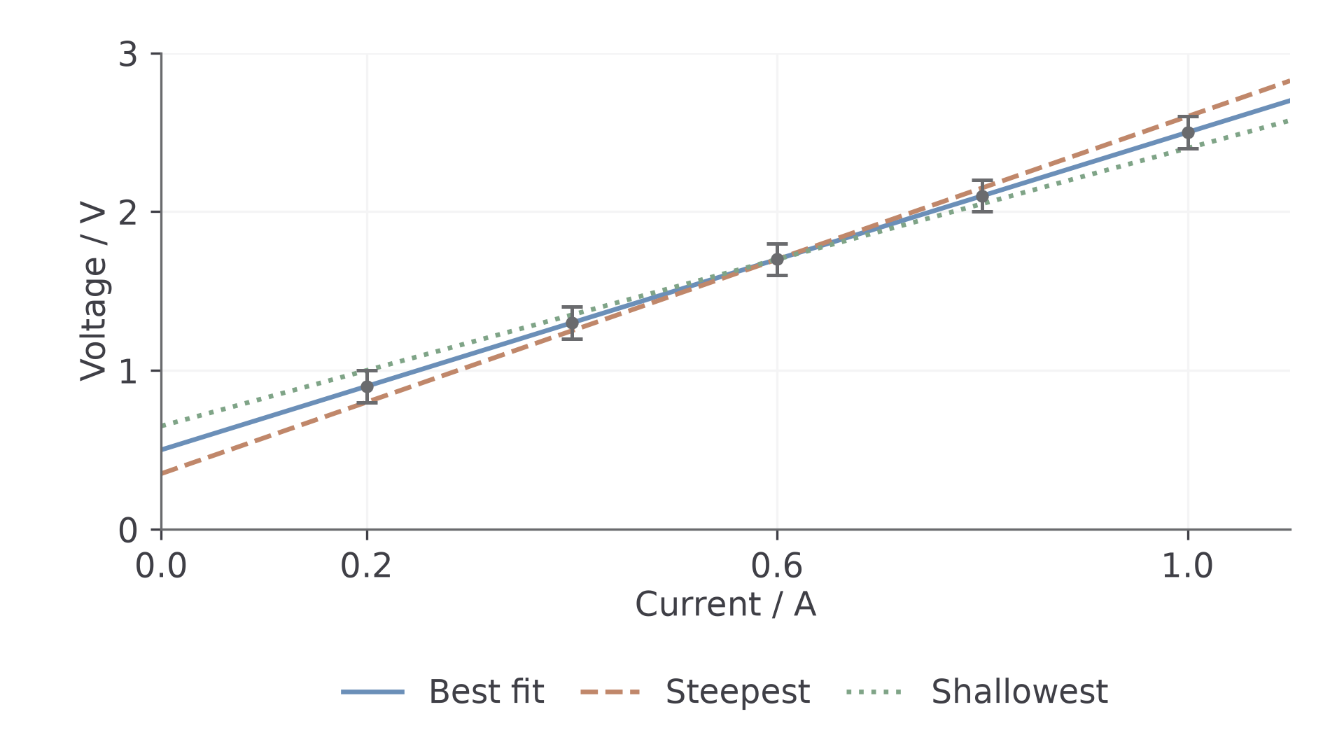
AQA's usual method compares the best fit with an acceptable extreme fit:
If both extremes are available, use the larger departure from the best gradient. In the plotted example, , and . Thus , or . The best intercept is ; the extremes are and , giving . Compare intercepts separately; the line with the largest gradient departure need not have the largest intercept departure in a general data set.
Use a half-range, , only when that convention is requested. It agrees with the best–worst method for symmetric bounds, but need not agree when the best gradient lies away from the midpoint. An intercept near zero is best reported with an absolute uncertainty, because its percentage uncertainty becomes unhelpfully large or undefined.
Choosing which uncertainty to reduce
A useful improvement targets the contribution that matters in the final calculation. The smallest raw measurement is not automatically the biggest problem: compare its fractional contribution after applying the relevant power.
Suppose , with exact constant . A 2% mass uncertainty and 1% diameter uncertainty each contribute 2% to , because the diameter is squared. Halving the mass uncertainty changes the total from 4% to 3%; halving the diameter uncertainty does the same. In contrast, improving an already tiny 0.1% contribution scarcely changes a much larger total.
Match the improvement to the cause. Use a wider measured interval when a nearly fixed reading uncertainty is dominant. Improve resolution only if resolution limits the measurement. Repeat independent measurements to investigate scatter, and sample different positions if the object is not uniform. More readings do not correct calibration bias or make a genuinely non-uniform wire uniform.
When a quantity comes from a graph, use the gradient's uncertainty as its contribution; do not then add the same underlying point uncertainties again. A wider data range can constrain the gradient more strongly, provided the same physical model remains valid over that range.
A measured result and a reference value agree within the stated uncertainty if their permitted ranges overlap. This supports consistency, not proof of an exact law. If the reference value has negligible uncertainty, check whether it lies inside the experimental interval. If it lies outside, investigate the model, systematic effects and uncertainty estimate.