3.13.3.2 - The Ideal Operational Amplifier

Signal inputs, output and supply connections

An operational amplifier, or op-amp, is a differential amplifier: it amplifies the difference between two input voltages. It is useful as a system building block because a circuit designer can use its input–output behaviour without analysing its internal transistors.

The non-inverting input is marked + and has voltage $V_+$. Increasing $V_+$ relative to the other input tends to increase the output. The inverting input is marked − and has voltage $V_-$. Increasing $V_-$ relative to the other input tends to decrease the output. These labels identify the response to a change; they do not mean that one input must always have a positive voltage and the other a negative voltage.

[DIAGRAM: asset_name: E.3.2 - The Ideal Operational Amplifier - Diagram 1; asset_slug: E.3.2 - The Ideal Operational Amplifier - Diagram 1; caption: The two signal inputs are separate from the positive and negative power supplies; description: Standard op-amp triangle with labelled non-inverting and inverting inputs, output and dual supply connections.]

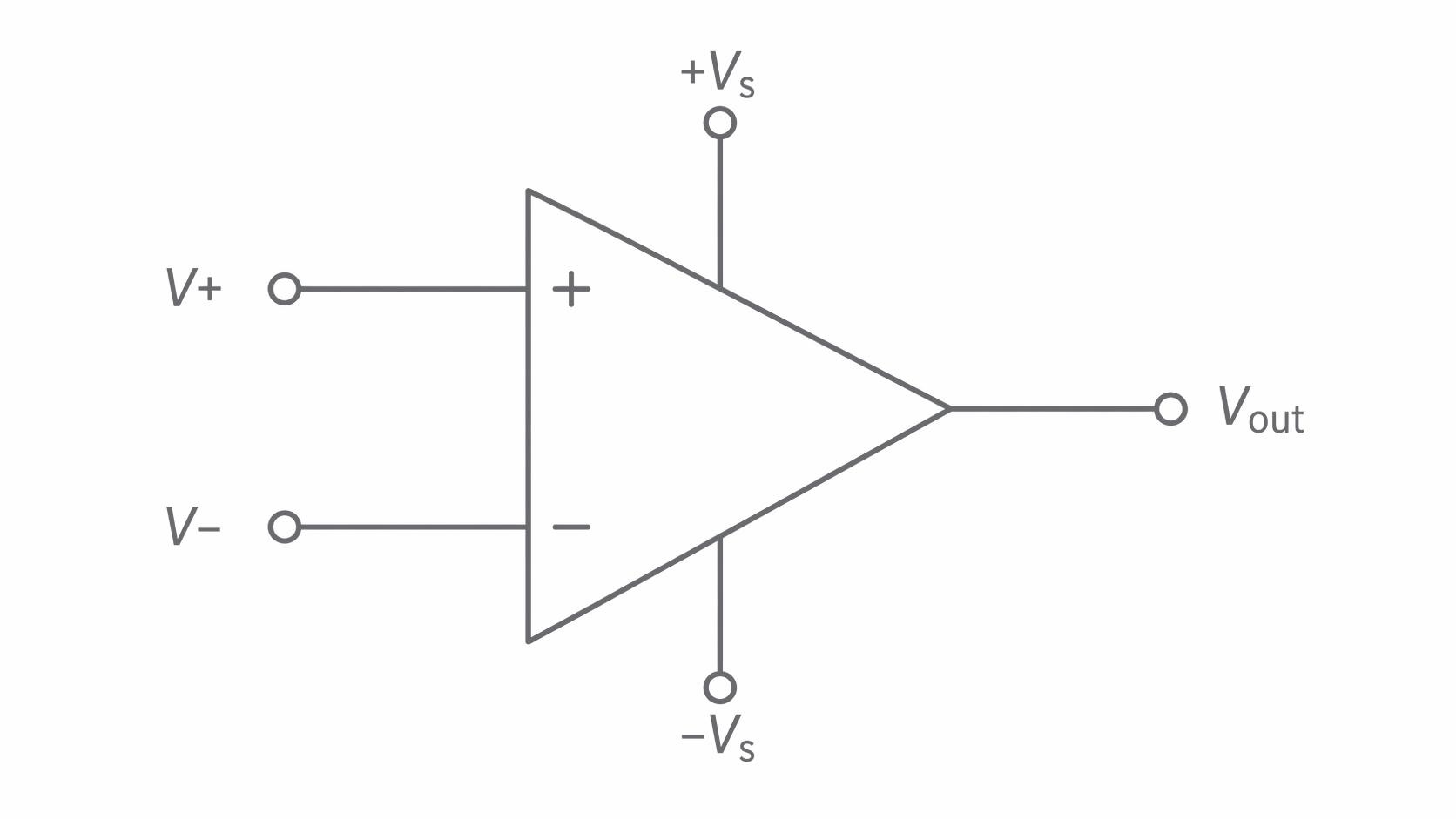
The supply connections provide the energy delivered to the output. In the diagram they are $+V_s$ and $-V_s$, measured from a common $0\,\mathrm{V}$ reference. They limit the possible output voltage. The input signals control the amplifier; they do not supply the output's energy.

A dual supply is common in examples, but an op-amp may instead use a single supply, such as $0$ and $+9\,\mathrm{V}$. Use the limits stated for the particular circuit. Never confuse a supply connection with the + or − signal input, even if the symbol is drawn with the input positions swapped.

The open-loop arrangement has no output signal fed back to an input. Its voltage gain refers to the differential input:

when the output is in its linear operating region. Gain is a dimensionless ratio, not a voltage.

Ideal gain and the absence of input loading

The ideal model uses infinite open-loop gain and infinite input resistance. Each assumption has a distinct consequence.

With infinite open-loop gain, any non-zero input voltage difference would demand an unlimited output from the linear equation. A powered amplifier cannot supply that: in open-loop comparator use it goes to the appropriate output limit. The ideal model therefore makes the transition between output states infinitely sharp. It does not predict an infinite delivered voltage.

Infinite input resistance means that no current enters either signal input. Connecting the input to a sensor divider therefore does not draw extra current from its junction and change the divider voltage. This is the absence of loading.

For example, a $6.0\,\mathrm{V}$ supply across two equal $10\,\mathrm{k\Omega}$ resistors gives a $3.0\,\mathrm{V}$ midpoint. Connecting an ideal op-amp input at that midpoint leaves it at $3.0\,\mathrm{V}$. A finite input resistance to ground would form a parallel path with the lower resistor and could reduce the midpoint voltage.

These assumptions concern the signal inputs. The op-amp can still draw supply current and deliver output current. Also, the two input voltages are not automatically equal in an ideal op-amp. They can differ in comparator use; equality is a condition used in particular negative-feedback analyses in later lessons.

Real open-loop gain and saturation

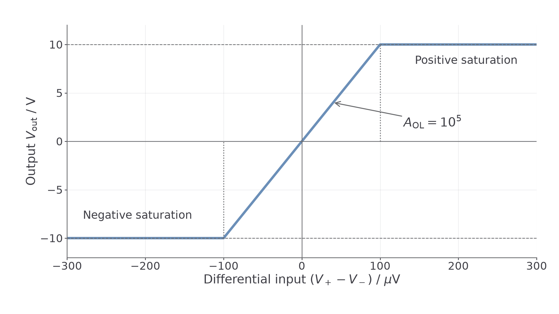
A real op-amp has a large but finite open-loop gain. In the narrow region where its output is not saturated,

Calculate the signed difference before multiplying. If $V_+>V_-$, the predicted output is positive; reversing that inequality reverses the sign. Both inputs can be positive while their difference is negative.

Saturation occurs when the linear formula would require an output beyond the amplifier's available range. A real output often stops short of the supply rail; use specified saturation voltages. Where a problem explicitly assumes saturation at the rails, clip the prediction to those rails. The finite-gain formula is not valid beyond saturation.

[DIAGRAM: asset_name: E.3.2 - The Ideal Operational Amplifier - Diagram 2; asset_slug: E.3.2 - The Ideal Operational Amplifier - Diagram 2; caption: A finite-gain transfer curve has a central linear region and two saturation regions; description: Exact curve for gain 100000 and assumed saturation at plus and minus 10 V, with differential input in microvolts and a central line through the origin.]