3.8.1.3 - Radioactive Decay

The random nature of radioactive decay and the decay constant

Radioactive decay is random: knowing the isotope does not let us predict when one particular nucleus will decay. It is spontaneous, requiring no external trigger. In the model used here, nuclei decay independently and the probability per unit time for an undecayed nucleus of a given isotope is constant. Ordinary laboratory changes of temperature or pressure do not appreciably change that probability.

A nucleus does not “age towards” its next decay. If it survives one half-life, its chance of surviving the next half-life is still one half. This memoryless behaviour applies to nuclei in the same radioactive state. The sample's activity nevertheless falls, because fewer undecayed nuclei remain available to decay.

The decay constant $\lambda$ describes the probability of decay per unit time for a surviving nucleus. Its SI unit is $\mathrm{s}^{-1}$. In a short interval $\Delta t$, for which $\lambda\Delta t\ll1$,

The minus sign describes a decrease in the number $N$ of undecayed nuclei. This is the instantaneous-rate model, or a short-interval approximation when written with finite differences. Do not use $\lambda t$ as a decay probability over a long interval: it could exceed one. The exact survival fraction over time $t$ is $e^{-\lambda t}$, so the decay probability is $1-e^{-\lambda t}$.

For example, if $\lambda=0.020\,\mathrm{s}^{-1}$, the probability of decay in the next $0.10\,\mathrm{s}$ is approximately $0.0020$, or $0.20\%$. The same value applies to a nucleus that has already survived for a minute. It does not guarantee that exactly $0.20\%$ of a small sample decays in that interval.

The exponential decay equation

Removing approximately the same fraction of the remaining nuclei in each equal time interval produces exponential decay. The expected number remaining is

Here $N_0$ is the initial number, and $\lambda t$ must be dimensionless: seconds must be paired with $\mathrm{s}^{-1}$, days with $\mathrm{day}^{-1}$, and so on. Because $N$ falls, the magnitude of the rate $\lambda N$ also falls. Exponential decay is not a constant number lost per second.

[DIAGRAM: asset_name: 8.1.3 - Radioactive Decay - Diagram 1; asset_slug: 8.1.3 - Radioactive Decay - Diagram 1; caption: A finite random-decay simulation fluctuates around the exponential expectation; description: Reproducible simulation and expectation for 80 nuclei with a four-second half-life. Stepwise whole-number losses are distinguished from the smooth expected population.]

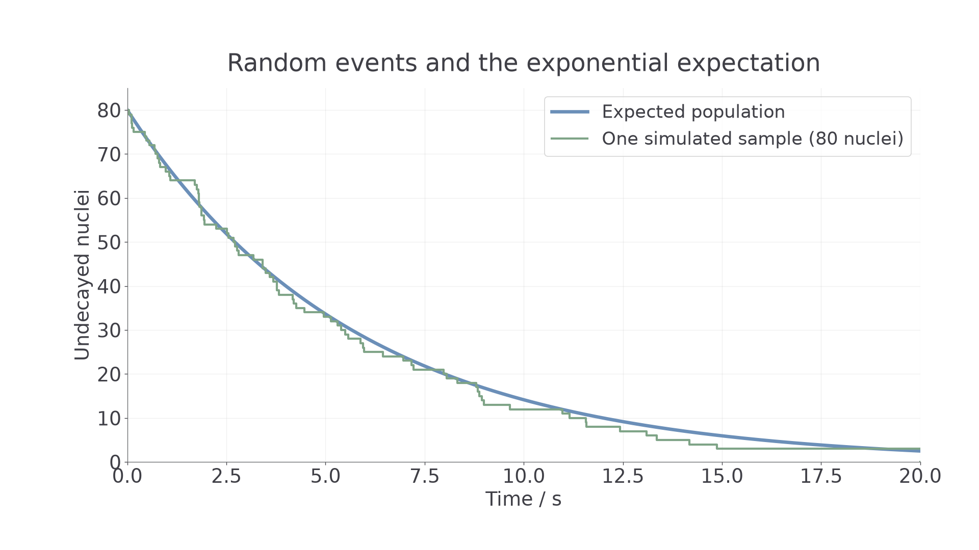
The smooth curve is an expectation, not a claim that actual counts change smoothly. A finite sample loses whole nuclei at random times and can eventually have none left. The mathematical expectation remains positive for finite time. Similarly, the mass of the parent isotope follows this law; the total mass of parent plus daughter material does not disappear at the same rate.

Modelling a constant probability

Shake many fair dice, remove those showing one, count the survivors, then repeat using only the survivors. Each die has probability $1/6$ of removal on each throw, independently of its earlier outcomes. For $k$ throws, the expected survivors are $N_0(5/6)^k$, but repeat runs fluctuate. With $600$ dice, the expected first two survivor counts are $500$ and $416.7$; an actual count must be an integer. A semilog plot is useful when counts span several orders of magnitude.

A spreadsheet can instead model small equal time steps with

For $N_0=1000$, $\lambda=0.020\,\mathrm{s}^{-1}$, $\Delta t=1.0\,\mathrm{s}$, the first expected approximations are $980$ and $960.4$. The exact value at $2.0\,\mathrm{s}$ is $1000e^{-0.040}=960.79$. Reducing the step improves the finite-difference approximation. It does not remove random variation from an actual experiment. A dice removal probability for a whole throw is not exactly the continuous decay constant; fitting $N=N_0e^{-\lambda_{\mathrm{eff}}k}$ gives $\lambda_{\mathrm{eff}}=-\ln(5/6)$ per throw.

Half-life

The half-life, $T_{1/2}$, is the time for the expected number of undecayed nuclei, or the activity, to fall to half its starting value. For a large sample this describes the observed trend closely. The same halving time applies whenever the measurement starts.

After $n$ half-lives, the expected fraction remaining is $2^{-n}$. After three half-lives, one eighth remains and seven eighths have decayed. To relate half-life to decay probability, substitute $N=N_0/2$ and $t=T_{1/2}$:

The initial population cancels, so the half-life is a property of the isotope and state, not the sample size. A large decay constant corresponds to a short half-life. Since $\ln2$ is dimensionless, $T_{1/2}$ has units of time.

For an isotope with half-life $5.0\,\mathrm{h}$, $\lambda=\ln2/(5.0\times3600)=3.85\times10^{-5}\,\mathrm{s}^{-1}$. After $15\,\mathrm{h}$, $12.5\%$ of the original nuclei remain; they do not have a different half-life because the sample is now older.

Activity

Activity $A$ is the decay rate of a radioactive sample, measured in becquerels: $1\,\mathrm{Bq}=1$ decay per second. It is positive even though the rate of change of undecayed population is negative:

Activity depends on both the number of radioactive nuclei and their decay constant. A short half-life gives a high activity for the same number of nuclei, but a large long-lived sample can be more active than a tiny short-lived one.

A detector's count rate is not generally the source activity. Only some emissions reach it, and only some of those are detected. After background subtraction, a fixed geometry and constant detection efficiency give $C_{\mathrm{net}}=\varepsilon A$, where $\varepsilon$ includes the detected fraction and emission yield. Count-rate ratios can therefore reveal decay without knowing $\varepsilon$, provided it stays constant. Moving the detector or allowing a daughter activity to build up can invalidate a simple single-exponential interpretation.