3.10.5.3 - Absorption of X-rays

Attenuation of the primary beam

Attenuation is a reduction in beam intensity as radiation passes through matter. Absorption transfers a photon's energy to the material. Scattering changes its direction, removing it from the original narrow beam even if it is not absorbed. An unscattered transmitted photon keeps its energy; attenuation does not mean every photon gradually loses energy or slows down.

[DIAGRAM: asset_name: B.5.3 - Absorption of X-rays - Diagram 1; asset_slug: B.5.3 - Absorption of X-rays - Diagram 1; caption: A photon can be transmitted, absorbed or scattered out of the primary beam; description: A photon can be transmitted, absorbed or scattered out of the primary beam.]

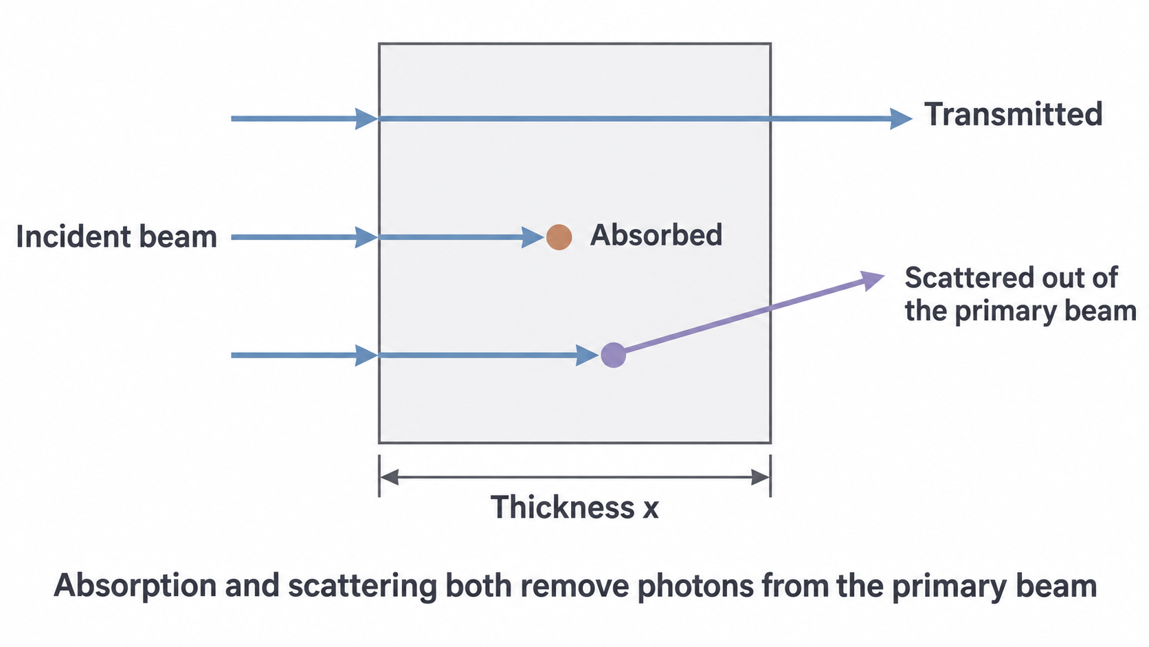
For a material of fixed composition and density, the removal probability depends on photon energy. Lower-energy photons are generally removed more strongly across much of the diagnostic range, but this is not an absolute law at every energy: material absorption edges can interrupt the trend. Compare supplied attenuation coefficients rather than guessing from energy alone.

The model conditions

A single constant attenuation coefficient describes a monoenergetic beam crossing a uniform material when scattered radiation is excluded from the measured primary beam. Keep source-detector geometry fixed so ordinary spreading of the beam is not mistaken for material attenuation. For a broad spectrum, low-energy photons are preferentially removed and the surviving beam hardens. The effective coefficient can then change with thickness.

Detailed atomic absorption and scattering mechanisms are outside this specification point. You need to distinguish their effects on the primary beam, not memorise a catalogue of interactions.

The exponential attenuation law

Each sufficiently thin layer of uniform material removes the same fraction of the photons reaching it. A later layer receives fewer photons, so it removes fewer in absolute number even though its removal probability is unchanged.

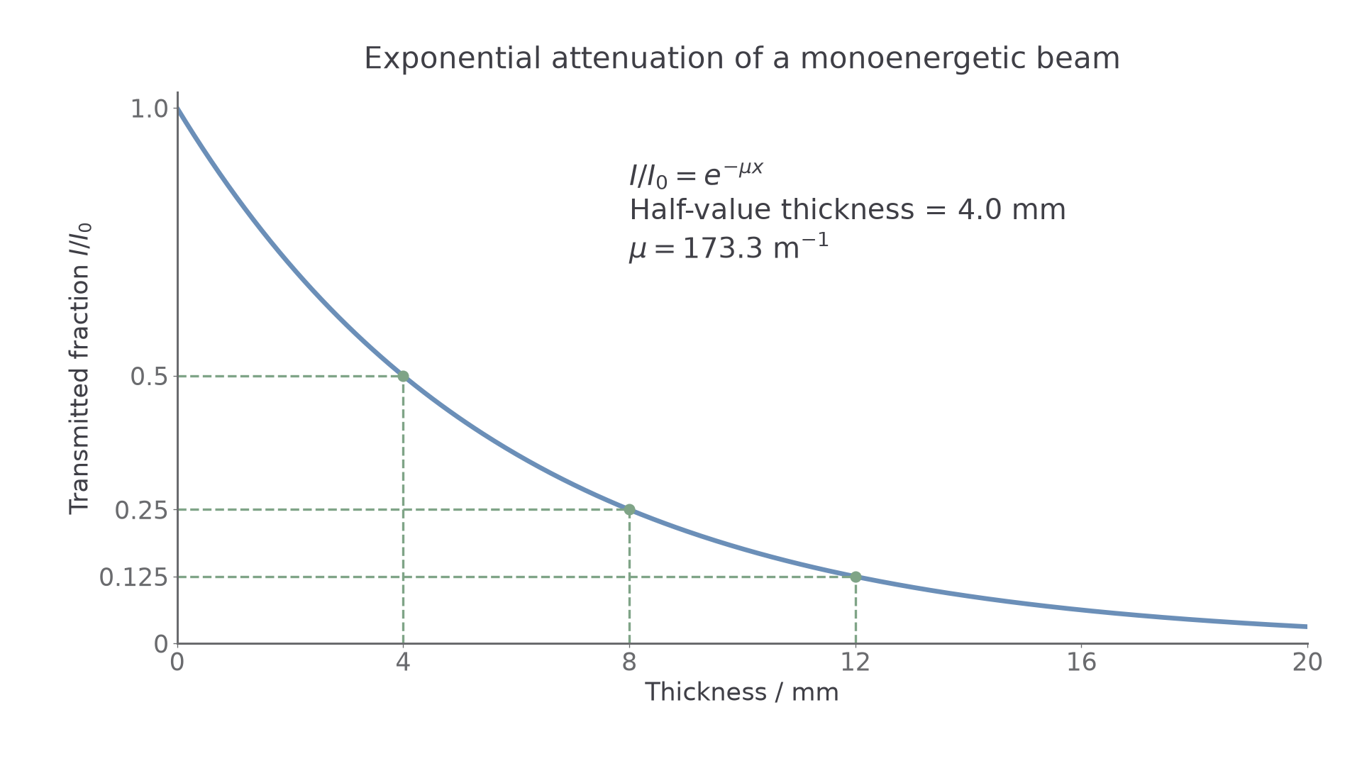
For a small thickness $\Delta x$, the fractional change is approximately $\Delta I/I=-\mu\Delta x$. The constant linear attenuation coefficient $\mu$ is the removal probability per unit path length, or the fractional intensity loss per unit thickness in the thin-layer limit. It is not the fraction removed by a whole metre of material.

The resulting law is

Here $I_0$ and $I$ are incident and transmitted intensities in $\mathrm{W\,m^{-2}}$, $x$ is path thickness in metres, and $\mu$ has units $\mathrm{m^{-1}}$. The exponent $\mu x$ must be dimensionless. A coefficient in $\mathrm{cm^{-1}}$ requires thickness in centimetres.

[DIAGRAM: asset_name: B.5.3 - Absorption of X-rays - Diagram 2; asset_slug: B.5.3 - Absorption of X-rays - Diagram 2; caption: A constant attenuation coefficient gives equal fractional losses in equal thicknesses; description: A constant attenuation coefficient gives equal fractional losses in equal thicknesses.]

Forward and inverse calculations

If $\mu=150\,\mathrm{m^{-1}}$ and $x=4.0\,\mathrm{mm}$, then $I/I_0=e^{-0.600}=0.549$. About $55\%$ is transmitted, not $60\%$ removed. The thin-layer approximation cannot be applied to an arbitrarily thick sample.

To infer the coefficient, rearrange using natural logarithms:

A plot of $\ln(I/I_0)$ against $x$ has gradient $-\mu$. The intensity ratio inside the logarithm is dimensionless. A straight line supports the constant-coefficient model; curvature can indicate a changing spectrum or other failures of the measurement assumptions. This is a data-analysis method, not an instruction to conduct an unsupervised X-ray experiment.

For separate layers, apply the law successively: $I=I_0e^{-\mu_1x_1}e^{-\mu_2x_2}=I_0e^{-(\mu_1x_1+\mu_2x_2)}$. Add exponents, not fixed amounts removed. This assumes the same monoenergetic primary beam model in each layer.