RP03 - Determination of g by Free Fall
Determine gravitational acceleration from measured fall distances and electronic timing. Choose a graph that matches the start of timing, then use scatter, instrument uncertainty and systematic effects to judge the result.
Choose a model that matches the timing
Required practical 3 measures by a free-fall method. In the timed region, use a dense ball, negligible air resistance and a nearly uniform gravitational field. Take downward as positive, so
Here is the displacement during the measured interval and is the velocity when that interval starts. It is not necessarily the velocity at release.
With two light gates, the ball falls some distance before it reaches the upper gate, so . Keeping release-to-upper-gate distance fixed keeps fixed. Rearranging gives
Plot vertically against horizontally. The gradient is in ; the intercept at is in . The graph's intercept must be free, not forced to zero.
If timing starts at physical release from rest and ends at impact, and . Then plotting against gives gradient . These are different measurements; inserting gate separation and gate-to-gate time into would give , which is too high.
Measure gate separation and transit time
Use a securely clamped stand, a low-voltage electromagnet or clean mechanical release, a dense steel ball, two light gates, an electronic timer or data logger, a metre rule and a padded catching tray. The upper gate starts timing when the ball interrupts its beam; the lower gate stops it using the same edge of the pulse.
[DIAGRAM: asset_name: RP 03 - Determination of g by a Free-Fall Method - Diagram 1; asset_slug: RP 03 - Determination of g by a Free-Fall Method - Diagram 1; recommended_method: retained_png; caption: Two-gate timing: h is the vertical separation of the beam levels. The ball already has velocity u at the upper gate.; description: Two-gate timing: h is the vertical separation of the beam levels. The ball already has velocity u at the upper gate.]
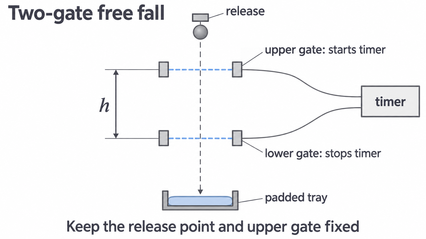
Fix the release point and upper gate. Align both beams under the release using a plumb line, then remove the line before dropping the ball. Make trial drops so the ball crosses both beams cleanly without striking a gate. Keep feet away from the drop zone; secure the stand and use a tray to prevent rebound.
Measure the vertical separation of the beam centres, using a ruler alongside the apparatus and a set square to transfer the levels. Read normal to the ruler to reduce parallax. Because the same part of the ball interrupts each beam, beam separation equals its displacement during the timed interval; do not measure magnet-to-lower-gate distance.
Record repeated times at each separation and calculate the mean after investigating any unusual result. Move only the lower gate to vary , for example through to in steps. Use a wider safe range if the apparatus allows. Preserve raw readings and units in the table rather than recording only a mean or calculated .
A timer resolving 1 ms does not necessarily have an uncertainty of exactly 1 ms. Check its specification and triggering behaviour. Data logging avoids hand reaction time, but good beam alignment and trigger settings still matter.
Controls and systematic timing effects
Vary the lower-gate position and measure transit time. Keep the release point and upper gate fixed so the entry velocity is constant. Keep the same ball and release procedure, and realign the lower gate after moving it. Changes in entry velocity between readings add scatter or distort the fitted line; they cannot always be represented by one new constant intercept.
Repeats help estimate scatter and reveal anomalies. An anomalous reading should be investigated and repeated, not deleted merely because it lies off a preferred line. Larger separations reduce the fractional effect of a fixed distance or timing uncertainty, but the ball must remain safely aligned and sufficiently far from terminal speed.
Release-to-impact timing
In the alternative method, measure the fall of the ball's bottom from its initial position to first contact with the impact switch. If the timer begins with the electrical release command and the ball detaches after a delay , the recorded time is . Then
Thus is too low. A plot of against is not exactly linear; a constant time offset is not simply a constant height intercept. Starting timing at actual release, measuring and correcting the delay, or switching to gate-to-gate timing addresses this bias. A mechanical release helps only if timing matches its actual release.
In the two-gate method a delay before the ball starts falling occurs before timing begins. By itself it does not lengthen the gate-to-gate time. A change in how the ball detaches can still change entry velocity, which is a different effect.
Processing data and finding the gradient
Use mean times to calculate a processed column. A spreadsheet can help, but inspect the formula, units, axes and fit; software does not decide the correct model. The original practice data below illustrate the two-gate method and are not claimed as measurements from a real experiment.
| Mean | ||
|---|---|---|
| 0.250 | 0.146 | 3.425 |
| 0.300 | 0.166 | 3.614 |
| 0.350 | 0.184 | 3.804 |
| 0.400 | 0.201 | 3.980 |
| 0.450 | 0.218 | 4.128 |
| 0.500 | 0.233 | 4.292 |
For the last row, . Do not round this column excessively before fitting.
[DIAGRAM: asset_name: RP 03 - Determination of g by a Free-Fall Method - Diagram 2; asset_slug: RP 03 - Determination of g by a Free-Fall Method - Diagram 2; recommended_method: retained_png; caption: Data and a free-intercept straight-line fit. The intercept is shown at t = 0, the enlarged data region makes the gradient readable.; description: Data and a free-intercept straight-line fit. The intercept is shown at t = 0, the enlarged data region makes the gradient readable.]
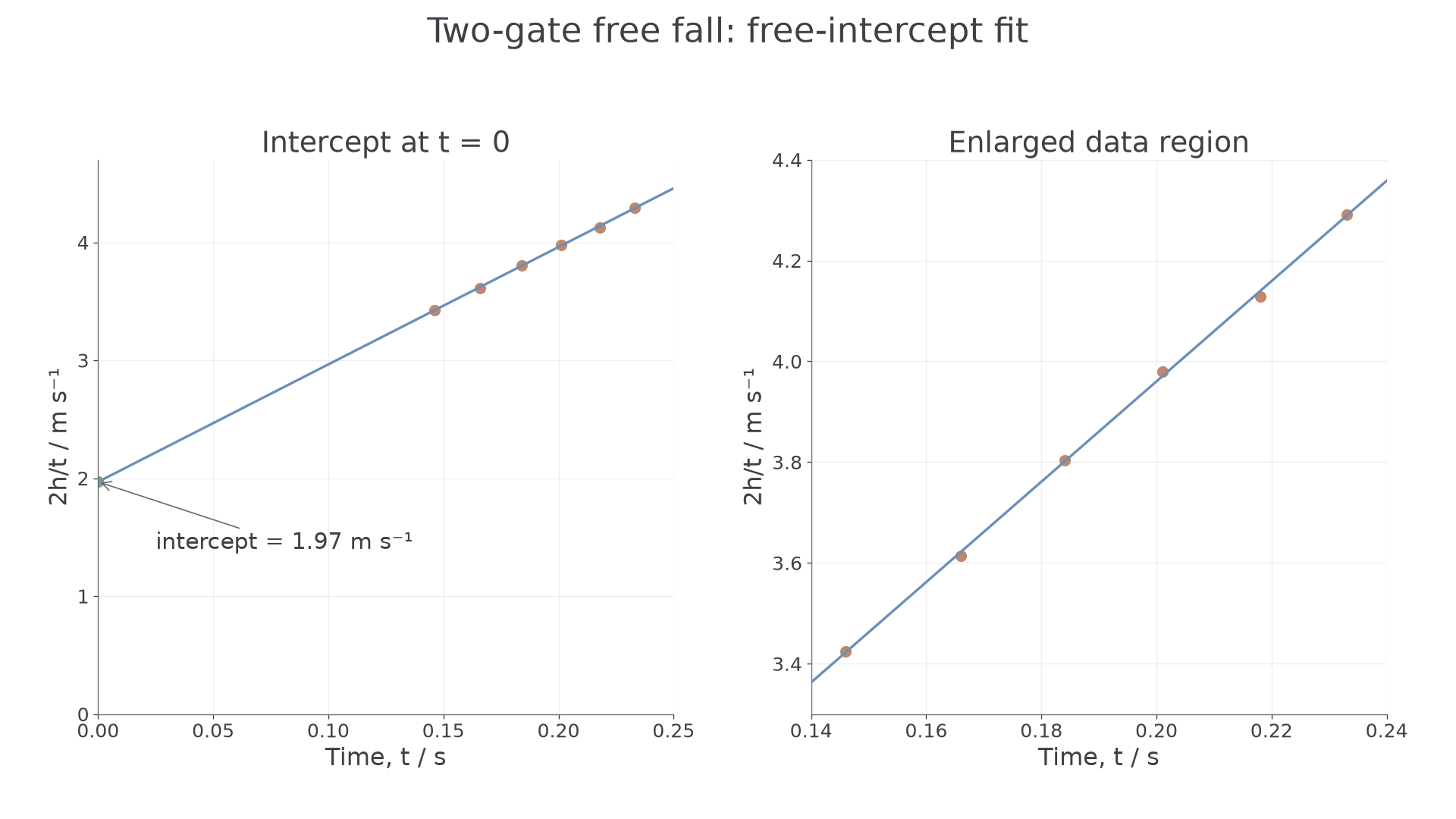
A least-squares line for these six processed points has gradient approximately and intercept . The gradient gives , and the intercept gives . A sensible hand-drawn fit may differ slightly.
When using a graph, select two widely separated points on the best-fit line and form ; do not automatically use the first and last measured points. Use the line equation if the intercept lies well outside the plotted data. Extrapolation makes the inferred intercept sensitive to gradient uncertainty.
For release-to-impact measurements from rest, choose against instead, and multiply its gradient by two. Expect the origin only for a correctly zeroed ideal model; inspect a free fit and residual pattern before forcing it through zero. A nonzero intercept can indicate a distance offset, while a time offset can cause curvature.
Uncertainty, scatter and bias
Uncertainty describes a justified range for a measurement; error is the unknown difference from the true value. Resolution is one source of uncertainty, not a guarantee of accuracy. Use at least half a division for one ideal analogue reading; two ruler readings each uncertain by give a minimum separation uncertainty of . Beam width, alignment and parallax may make it larger.
For repeated times , the mean is and half-range is . Compare this with resolution and manufacturer/trigger uncertainty; do not claim zero uncertainty just because repeated displayed readings match. Repeats estimate scatter and can improve the mean, but do not remove systematic offsets.
For a product or quotient, add fractional uncertainties; powers multiply them. The factor 2 is exact:
For , , the percentage uncertainty in is . For in a genuine release-from-rest method, it would instead be .
Draw relevant error bars and a best-fit line. Estimate gradient uncertainty from the largest difference between the best gradient and a steepest or shallowest acceptable line, following the stated task convention. If and the worst acceptable gradient is , quote , or . Do not substitute a single data point's percentage uncertainty for gradient uncertainty. In the two-gate graph, time appears on both axes, so its uncertainties are correlated; a simple fit is an A-level estimate, not evidence of fully independent x and y errors.
Parallax can be systematic if the eye is consistently misplaced, or contribute random scatter if the viewpoint varies. Air drag is a systematic departure from the free-fall model: use a dense ball and a suitable drop range. A fixed height zero error shifts measured separations; check the actual beam levels. Classify the mechanism in the stated setup rather than labelling every ruler error random.
Judging consistency and improving the method
Compare the measured and its justified uncertainty interval with a reference value. For , the interval is to , which includes . The result is consistent within this uncertainty; it does not prove that every systematic error has been removed.
Also inspect the pattern: approximate linearity supports constant acceleration with fixed entry speed. A plausible positive intercept supports the two-gate interpretation . Curvature, a changing intercept between runs or systematic residuals can reveal an inadequate model or control. A precise but biased result may have little scatter yet disagree with the reference; a broad interval is not evidence of high precision.
An evaluation should link a specific limitation to a measurable effect and a feasible improvement. For example, a fixed release delay makes release-to-impact times too long; start timing at physical release or use two gates. A narrow separation range makes the fitted gradient more sensitive to reading errors; extend the safe range while preserving alignment and negligible drag. Neither improvement is captured by simply saying “use better equipment”. When reporting your practical, cite the AQA practical handbook for the chosen method and identify the timer manufacturer’s specification used for timing uncertainty. Distinguish your own recorded data from illustrative or published results.