3.13.2.1 - Analogue and Digital Signals
A microphone produces a continuously varying voltage, but a digital link sends a sequence of bits. Learn how sampling and quantisation connect these representations, what limits the recovered sound quality, and why recognisable digital pulses can be regenerated after transmission.
Signals from sensors
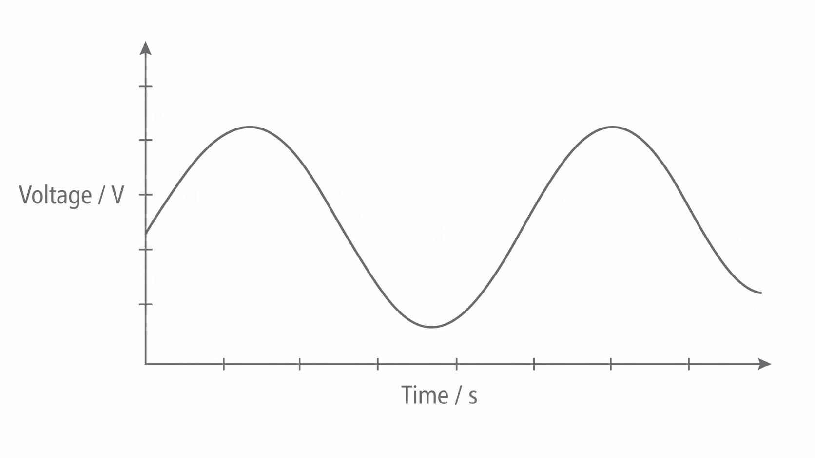
An analogue signal represents a changing physical quantity by an electrical quantity that can take any value within a continuous range. A microphone, for example, converts sound-pressure variations into voltage variations. Its voltage is not restricted to a fixed list of values.
Sensors collect many kinds of analogue data. A thermistor changes resistance with temperature; an LDR changes resistance with light intensity. A potential divider converts either resistance change into a voltage. A photodiode produces a light-dependent current, while a Hall sensor can provide a voltage related to magnetic field strength. The sensor and its circuit must be considered together: a resistance sensor does not generate a voltage by itself.
[DIAGRAM: asset_name: E.2.1 - Difference Between Analogue and Digital Signals - Diagram 1; asset_slug: E.2.1 - Difference Between Analogue and Digital Signals - Diagram 1; caption: An analogue voltage can take any value within its range; description: Qualitative voltage-time waveform with continuous amplitude. Tick marks are unnumbered and no quantitative readings are intended.]
A binary digital signal represents information using two recognised states, logic 0 and logic 1. These might be nominal voltages of and . A real pulse takes time to change level and may carry noise; the receiver interprets it as one of the two states. It is the allowed information states, rather than a physically instantaneous voltage jump, that distinguish the digital representation.
[DIAGRAM: asset_name: E.2.1 - Difference Between Analogue and Digital Signals - Diagram 2; asset_slug: E.2.1 - Difference Between Analogue and Digital Signals - Diagram 2; caption: Binary pulses use two nominal voltage levels; description: Idealised rectangular pulses switching between labelled 0 V and 5 V states.]
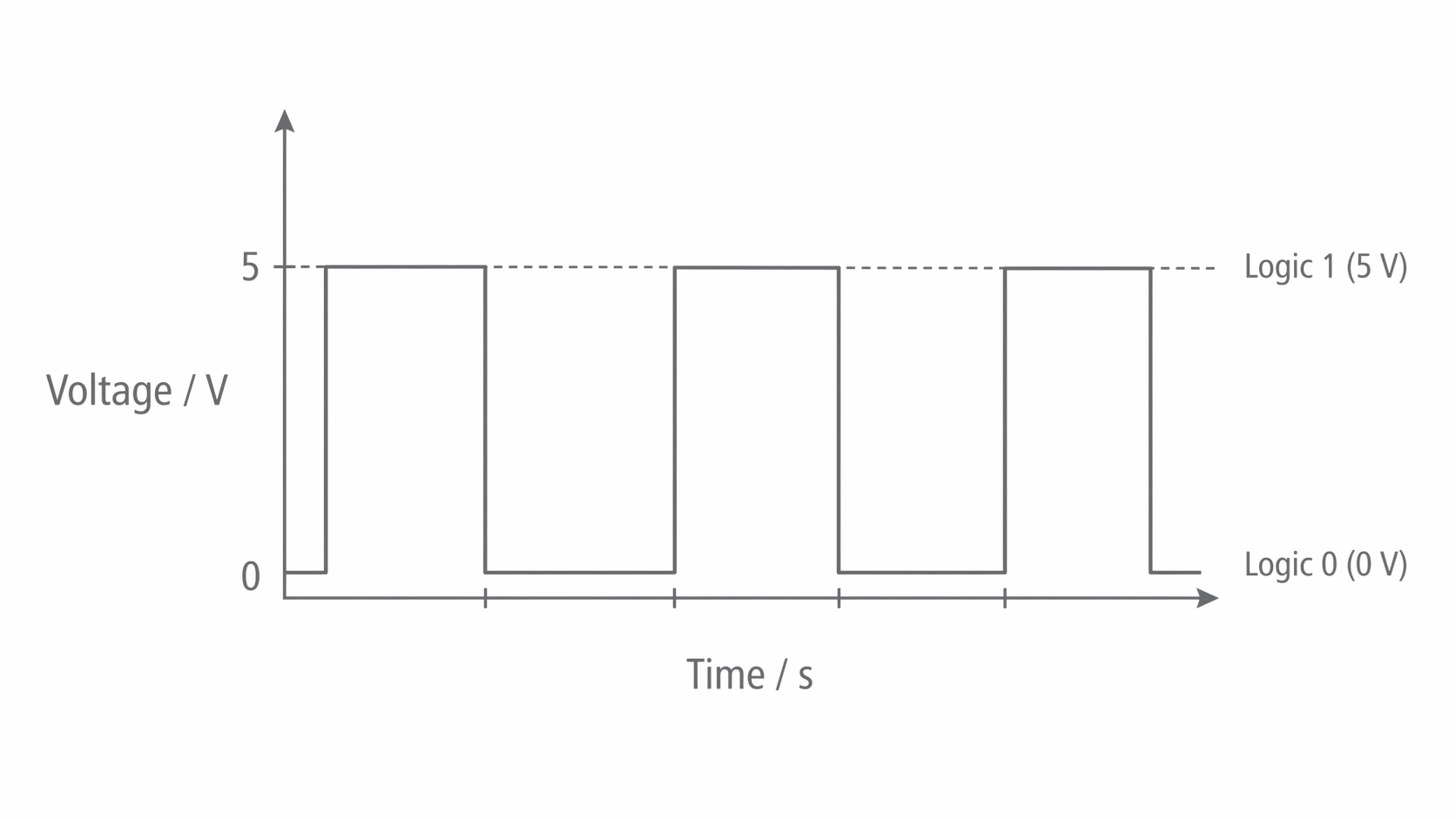
The voltage does not itself mean that a sampled sound has amplitude 5. It represents one bit. Several consecutive bits encode the measured amplitude.
Bits, bytes and sample codes
A bit is a binary digit, 0 or 1. A byte contains eight bits. With bits there are different possible codes: each extra bit doubles the number of choices. Thus a byte has 256 possible codes, even though each transmitted bit still uses only two voltage states.
For four-bit numbers the place values, from left to right, are 8, 4, 2 and 1. For example, 1010 represents . Leading zeros do not change the value.
| Decimal | Binary | Decimal | Binary |
|---|---|---|---|
| 0 | 0000 | 6 | 0110 |
| 1 | 0001 | 7 | 0111 |
| 2 | 0010 | 8 | 1000 |
| 3 | 0011 | 9 | 1001 |
| 4 | 0100 | 10 | 1010 |
| 5 | 0101 |
Knowledge of binary numbers 1 to 10 is sufficient for this topic; binary arithmetic is not required. Zero is included to show the lowest code.
To compare a data rate in bits per second with one in bytes per second, divide by eight. For example, 600 samples, each containing eight bits, require bits or bytes before any extra transmission information is added.
Sampling, quantisation and pulse code modulation
An analogue-to-digital converter (ADC) measures the input voltage at separate instants and produces codes representing those measurements. In pulse code modulation (PCM) the sequence of amplitude codes is transmitted as binary pulses.
The three operations answer different questions:
- Sampling: what is the signal voltage at this instant? Measurements are taken at regular time intervals.
- Quantisation: which allowed amplitude level represents this measurement? In a nearest-level converter, the measured value is rounded to the nearest available level.
- Encoding: which binary code identifies that level? The code is then sent using high and low pulses.
[DIAGRAM: asset_name: E.2.1 - Difference Between Analogue and Digital Signals - Diagram 3; asset_slug: E.2.1 - Difference Between Analogue and Digital Signals - Diagram 3; caption: Equal-time samples are rounded to levels and assigned consistent binary codes; description: Exact plotted example with sample instants 0 to 5 ms, levels 0 to 3 V, two-bit codes 00 to 11 and independently marked measured and quantised values.]
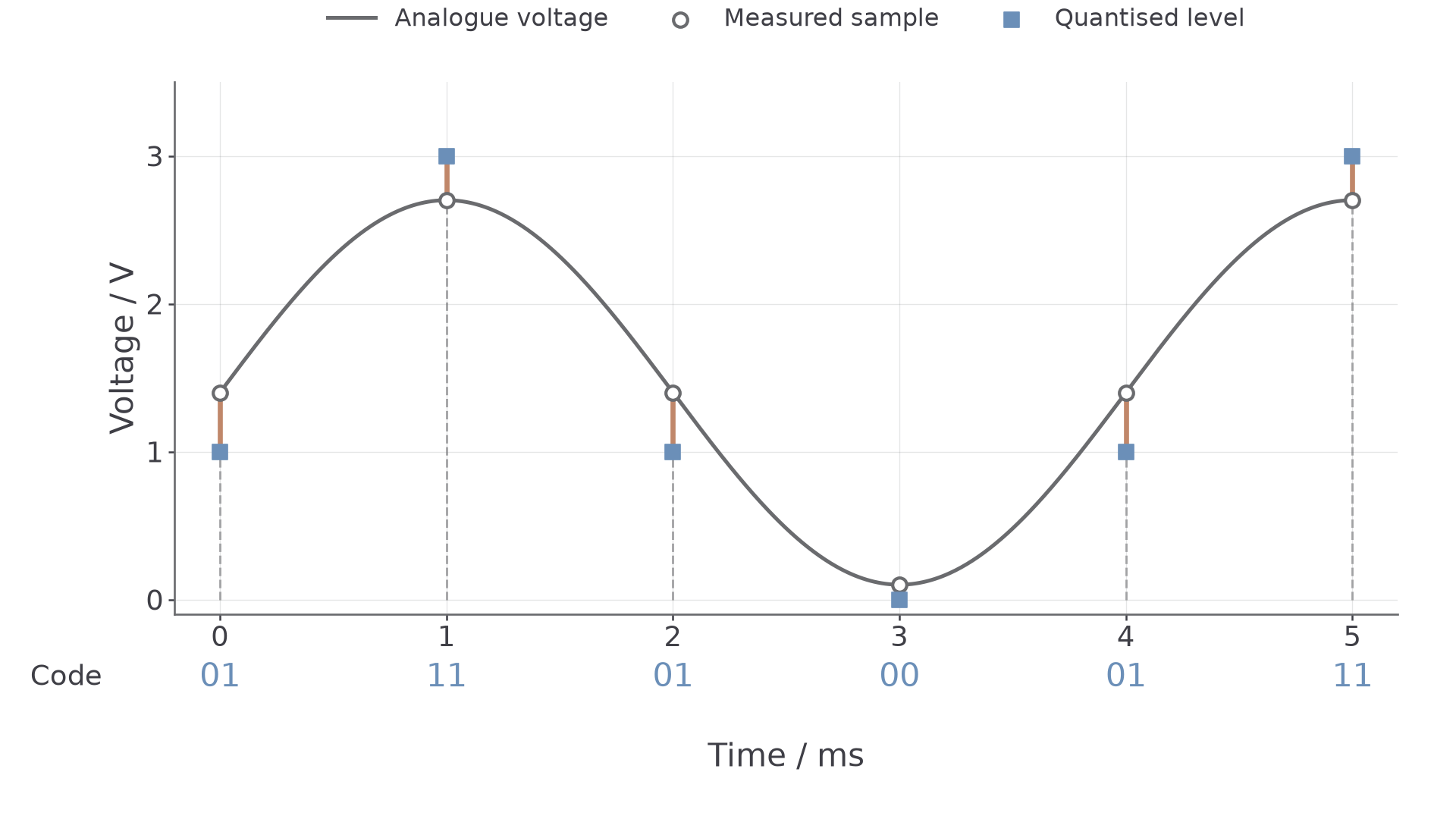
In the figure, the sample near is represented by the level and code 11. The rounded amplitude is an approximation; the transmitted high/low voltages encode the code, not the original waveform shape.
Time resolution and amplitude resolution
The sampling rate is the number of samples per second. The sampling interval is . A rate of , for example, gives an interval of .
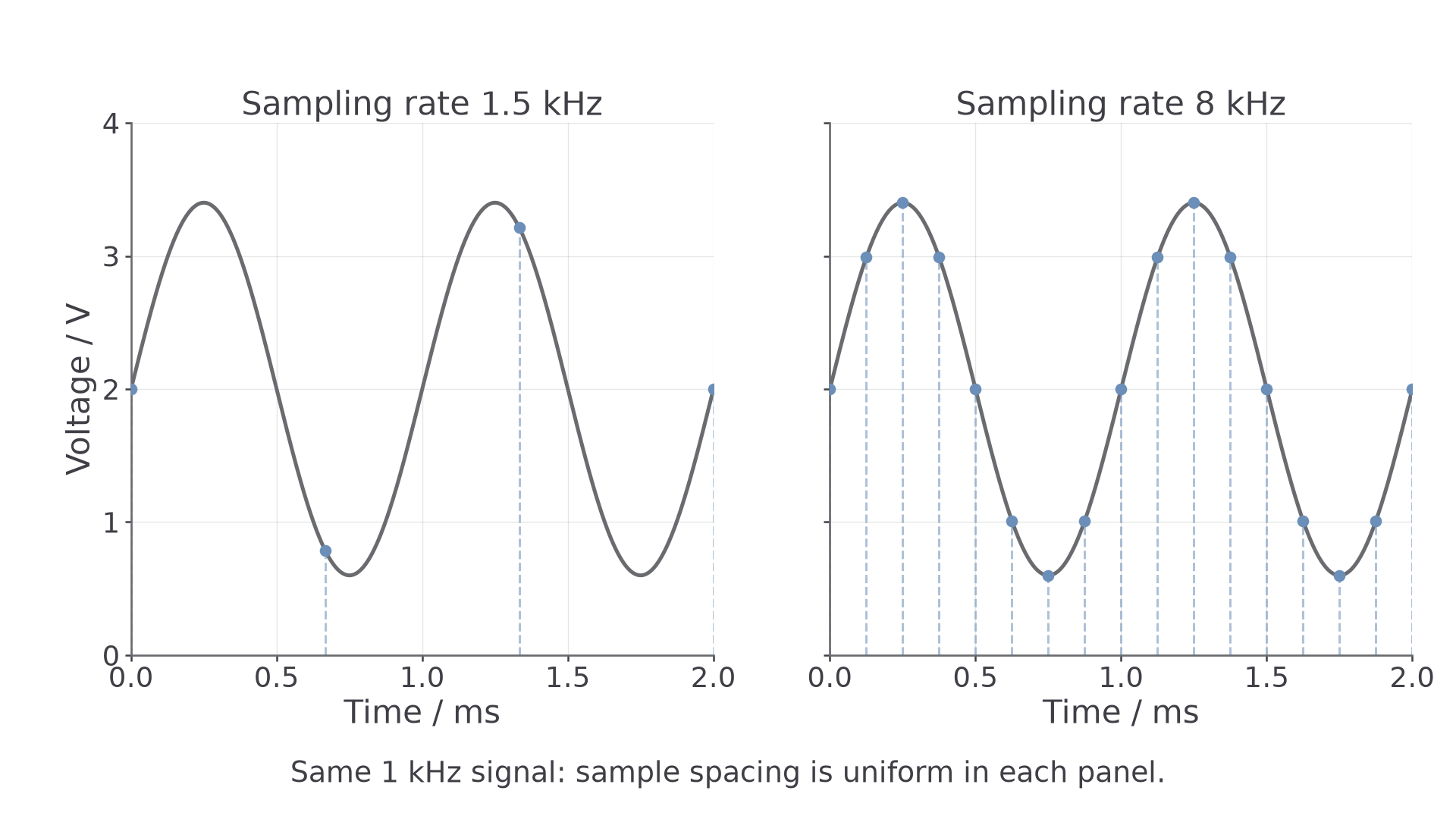
Sampling too slowly can make a rapidly varying signal appear to vary more slowly: aliasing. The usual minimum-rate criterion is twice the highest signal frequency. Practical sampling uses a rate above this limit and limits the frequencies entering the ADC; exact equality can be ambiguous for particular sampling phases. Increasing an already adequate rate does not remove amplitude-rounding error.
[DIAGRAM: asset_name: E.2.1 - Difference Between Analogue and Digital Signals - Diagram 4; asset_slug: E.2.1 - Difference Between Analogue and Digital Signals - Diagram 4; caption: The same waveform sampled at equal intervals at two different rates; description: Exact plots of a 1 kHz voltage waveform with 1.5 kHz and 8 kHz sample rates. Sample points lie on the same waveform and have uniform time spacing.]
For a fixed input range, more bits per sample provide more quantisation levels and smaller voltage steps. A specified uniform ADC with equal bins over range has step size
Use the grid or convention supplied in a question: a list of levels including both endpoints can have a different number of intervals. A voltage change smaller than one step may change the code if it crosses a decision boundary; the step is not a guarantee that every smaller change is invisible.
Continue this lesson.
You’re previewing NovaLearn without an account. Create a free account to read the rest.
Create free account