3.12.2.3 - Electromagnetic waves

Fields that travel together

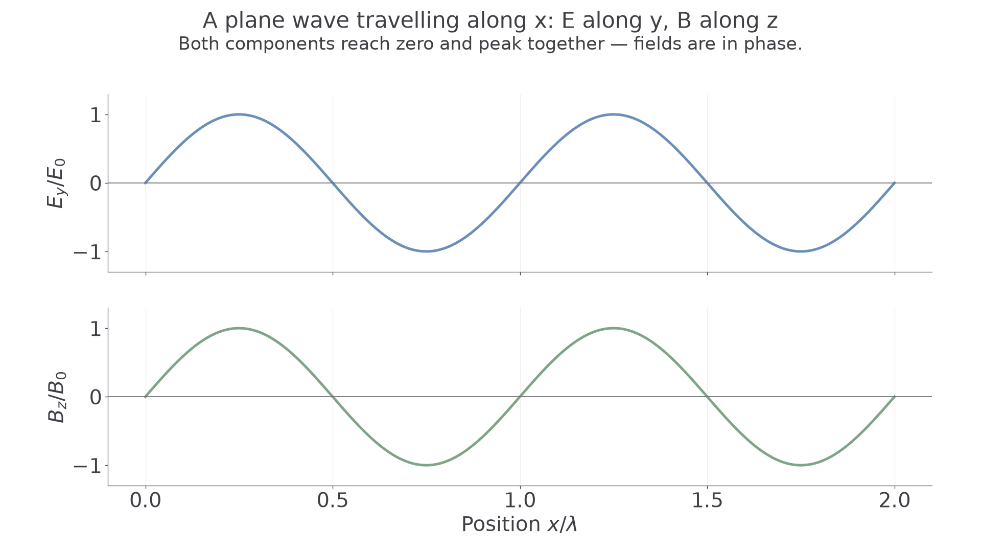
An electromagnetic wave carries energy through oscillating electric and magnetic fields. In a plane wave in free space, the fields are perpendicular to each other and to the direction of propagation. Both are therefore transverse. They oscillate in phase: at a given position their maxima, minima and zeros occur together.

The graph represents field components against position at one instant. Its vertical axes are normalised separately; electric field strength and magnetic flux density have different units. The curves do not represent a wavy path followed by particles. At each point the fields change with time while the wave pattern travels forward.
[DIAGRAM: asset_name: D.2.3 - Electromagnetic Waves - Diagram 1; asset_slug: D.2.3 - Electromagnetic Waves - Diagram 1; caption: Electric and magnetic field components vary in phase along a plane wave; description: Scientific teaching diagram with geometry and labels checked against the owning explanation.]

Electromagnetic waves need no material medium and can travel in a vacuum. For a linearly polarised wave, the electric field oscillates in one fixed transverse direction. A receiving dipole responds most strongly when aligned with that electric field. Rotating it about the propagation direction through a right angle reduces the response to a minimum. This is evidence for transverse oscillations; polarisation alone does not identify a wave as electromagnetic, since other transverse waves can also be polarised.

Maxwell's quantitative prediction

Maxwell's equations linked electric and magnetic phenomena and predicted electromagnetic waves with a definite speed in free space:

Permittivity $\varepsilon_0$ relates charge to its electric field in free space. For example, at distance $r$ from an isolated point charge $Q$, $E=Q/(4\pi\varepsilon_0r^2)$. Permeability $\mu_0$ relates current to magnetic flux density in free space: for a long straight wire, $B=\mu_0I/(2\pi r)$. These examples explain what the constants describe; the option does not require a derivation of Maxwell's equations.

Using the exam values $\varepsilon_0=8.85\times10^{-12}\,\mathrm{F\,m^{-1}}$ and $\mu_0=4\pi\times10^{-7}\,\mathrm{H\,m^{-1}}$, their product is approximately $1.112\times10^{-17}\,\mathrm{s^2\,m^{-2}}$. Its square root is $3.335\times10^{-9}\,\mathrm{s\,m^{-1}}$, giving

The square root applies to the entire product. The crucial result is not just this arithmetic: a speed derived from electromagnetic quantities agreed with the independently measured speed of light. That agreement suggested that light is an electromagnetic wave. Maxwell predicted the speed of electromagnetic waves; he did not determine it by timing a light beam.

Hertz: production, detection and speed

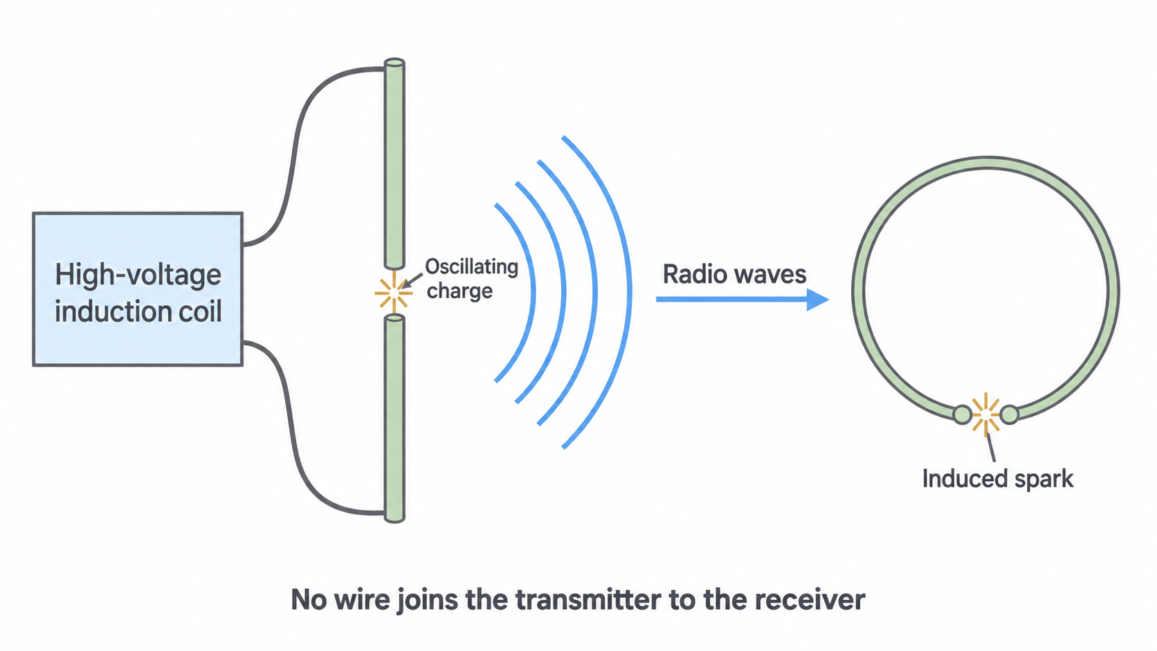
Hertz generated radio waves using a spark-gap transmitter. A high-voltage induction coil charged conductors on either side of a small gap; the discharge produced rapidly oscillating charges. Accelerating charges radiate electromagnetic waves. A separate receiving loop with a small gap showed a tiny induced spark: energy had reached the receiver without a connecting wire.
[DIAGRAM: asset_name: D.2.3 - Electromagnetic Waves - Diagram 2; asset_slug: D.2.3 - Electromagnetic Waves - Diagram 2; caption: Hertz’s separate transmitter and receiver demonstrate radio-wave transfer; description: Scientific teaching diagram with geometry and labels checked against the owning explanation.]

Hertz investigated reflection, refraction, interference and polarisation of the radiation. These observations established wave behaviour and were consistent with the electromagnetic theory. For a suitably oriented loop, changing magnetic flux induces an emf; a dipole responds to the electric field. Detector orientation matters, so a weak response need not mean no wave is present.