RP05 - Determination of Wire Resistivity
Determine a wire’s resistivity by combining its diameter with a resistance–length graph. Plan measurements that test the uniform-wire model, then quantify what the uncertainty permits you to conclude.
Why a resistance–length graph gives resistivity
For a uniform wire at a fixed temperature, . Resistance depends on the specimen; resistivity characterises its material under those conditions. Its unit is .
Measure for several lengths of the same wire. A graph of vertically against horizontally should have gradient , so
Here is diameter, not radius, and must be converted to metres before squaring. The ideal intercept is zero; a fitted intercept is also useful evidence about systematic effects.
Constantan is a suitable example because a school-length specimen has a readily measurable resistance and its resistance changes relatively little with temperature. These are advantages, not a guarantee that heating or contact effects vanish. A different wire material is acceptable if its geometry, resistance and safe measuring current suit the instruments.
A gradient of does not itself give resistivity. For diameter , , hence . A thinner wire of the same material would have a larger gradient.
Measuring diameter and constructing the circuit
The length used in the calculation must be the same wire section across which the pd is measured. Use a low-voltage DC supply, current-limiting resistance, switch, ammeter, high-resistance voltmeter, ruler, micrometer and suitable wire contacts.
[DIAGRAM: asset_name: RP 05 - Determination of Resistivity of a Wire - Diagram 1; asset_slug: RP 05 - Determination of Resistivity of a Wire - Diagram 1; caption: The test wire completes the supply loop. Its voltage-sensing endpoints A and B also define the measured length. The ammeter reads supply current, approximately wire current when voltmeter loading is negligible.; description: The test wire completes the supply loop. Its voltage-sensing endpoints A and B also define the measured length. The ammeter reads supply current, approximately wire current when voltmeter loading is negligible.]
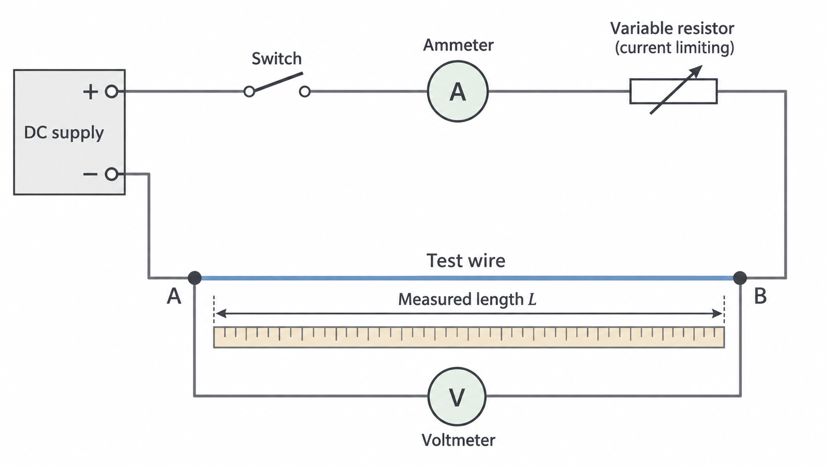
Build the supply, switch, ammeter, limiter and wire in series. Add the voltmeter across only the selected wire length. Check polarity and meter ranges before closing the switch; an ammeter connected across the supply would create a low-resistance path. Start with the supply low and current-limiting resistance high. Keep within wire, resistor and meter ratings. Open the switch before moving clips; hot fine wire can burn and sharp cut ends need careful handling.
[DIAGRAM: asset_name: RP 05 - Determination of Resistivity of a Wire - Diagram 2; asset_slug: RP 05 - Determination of Resistivity of a Wire - Diagram 2; caption: Micrometer parts with jaws open before measurement. Close the anvil and spindle gently onto the wire using the ratchet. This illustration is not a diameter reading.; description: Micrometer parts with jaws open before measurement. Close the anvil and spindle gently onto the wire using the ratchet. This illustration is not a diameter reading.]
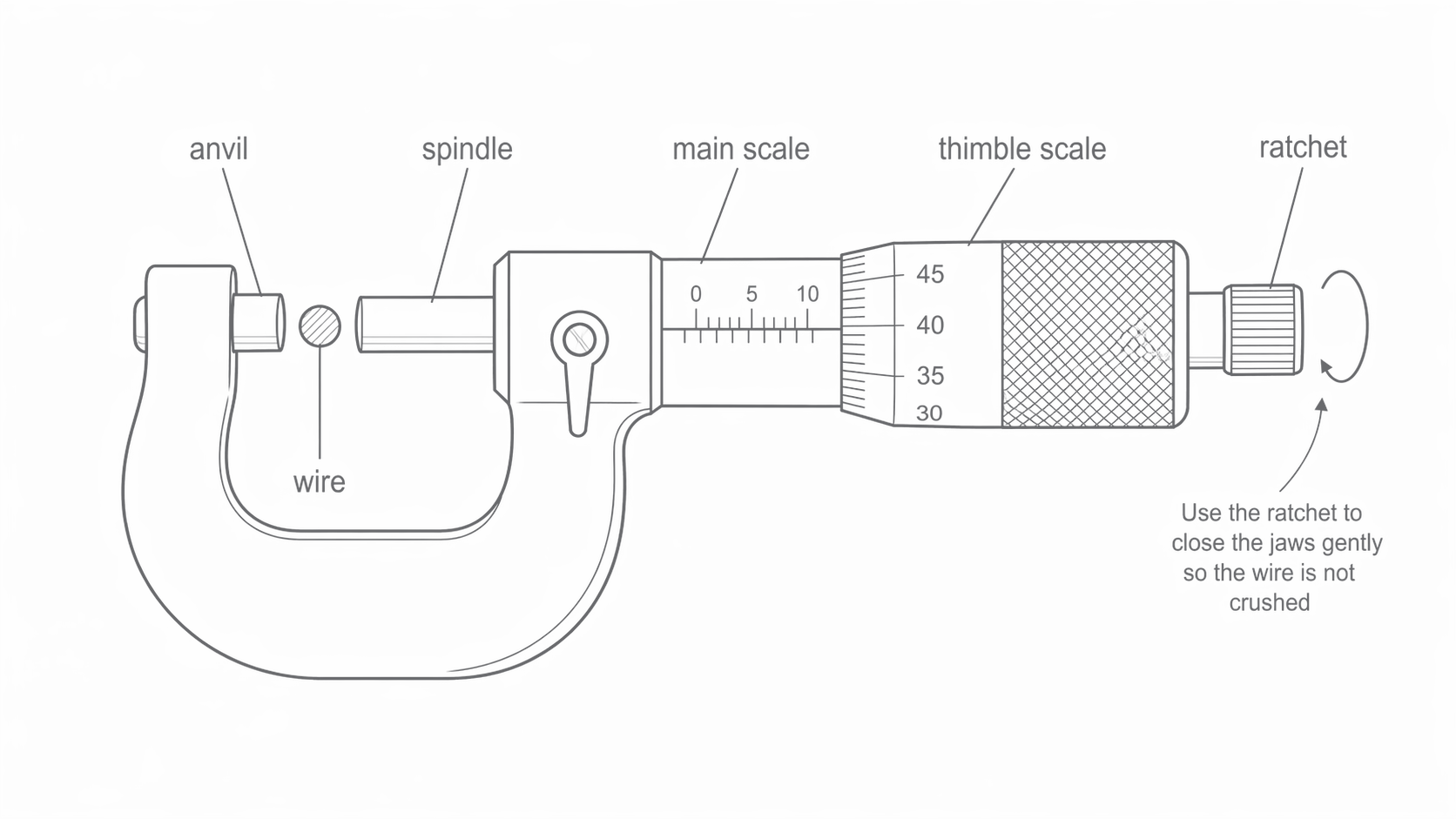
Check the closed-jaw zero with the ratchet, record the offset and subtract it from each reading. Read the last visible main-scale mark and add the thimble contribution. For example, on the main scale plus on the thimble gives ; a zero offset makes the corrected diameter . For a digital instrument, record its displayed value and resolution and still check zero.
Measure diameter at several positions and rotate the wire to check ovality. Use the ratchet consistently rather than squeezing the wire. Record all readings before calculating a representative corrected mean. Keep the wire straight alongside the ruler without stretching it; measure between the actual contact points and view the scale perpendicularly.
Choosing a range and controlling heating
Vary the length ; the dependent quantity is resistance calculated from paired and readings. Keep material and cross-section the same by using one suitable wire, and keep its temperature approximately constant. Clean, firm contacts reduce unstable readings.
Choose several lengths across a wide usable range. Very short lengths may have poor fractional length and pd precision; very long lengths may exceed the ruler or supply range. Pilot readings help choose a range with a measurable change in while current remains safe. A fixed current is convenient but not essential: record the actual and together and calculate their ratio for every measurement.
For each measured length, close the switch briefly, record a stable pair, then open it. Limit current to avoid appreciable heating; the appropriate current depends on the wire and apparatus, so is not a universal prescription. If readings drift while the switch is closed, lower the current or allow longer cooling. Repeat the measurements and compare the repeated values before averaging. Revisit an earlier length near the end to test for time-dependent drift.
Maintain a raw table with units in column headings, all repeats, corrected diameters, actual lengths and instrument details. Do not silently replace an unexpected result. Record the reason for remeasurement or any justified exclusion. This record allows someone else to distinguish scatter from an uncontrolled change in conditions.
Fitting the graph and interpreting an intercept
Calculate each resistance before fitting the graph. The following is an original illustrative dataset for a wire measured at approximately , not a reproduction of official experimental results.
| 0.10 | 0.204 | 0.200 | 1.02 |
| 0.20 | 0.396 | 0.200 | 1.98 |
| 0.30 | 0.604 | 0.200 | 3.02 |
| 0.40 | 0.800 | 0.200 | 4.00 |
| 0.50 | 1.004 | 0.200 | 5.02 |
| 0.60 | 1.196 | 0.200 | 5.98 |
| 0.70 | 1.400 | 0.200 | 7.00 |
| 0.80 | 1.604 | 0.200 | 8.02 |
[DIAGRAM: asset_name: RP 05 - Determination of Resistivity of a Wire - Diagram 3; asset_slug: RP 05 - Determination of Resistivity of a Wire - Diagram 3; caption: The plotted points match the illustrative table. A best-fit line and widely separated line coordinates give a gradient close to 10.0 ohm per metre.; description: The plotted points match the illustrative table. A best-fit line and widely separated line coordinates give a gradient close to 10.0 ohm per metre.]
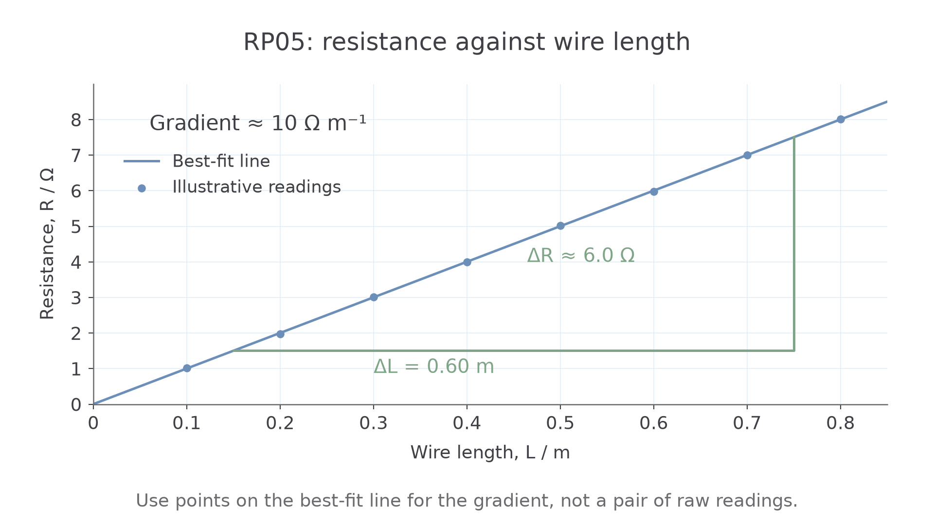
Use labelled axes, sensible scales and an overall best fit; do not join every point or force the origin. On paper a large gradient triangle reduces read-off error. A spreadsheet linear fit is an alternative, but its coefficients need units and a physical interpretation. Inspect the residual pattern rather than accepting a fit automatically.
If , an included constant contact resistance raises the intercept without changing . Dividing one by then overestimates the gradient. This explanation applies only to resistance included between the voltage-sensing points; supply leads outside them do not directly contribute. An intercept can also arise from a length offset. Its size must be compared with measurement uncertainty before claiming a systematic error.
Repeat and investigate a suspect datum. If repeated values consistently show the same departure, the model may be inadequate: deleting them is not justified merely because the line looks neater. Variable contact resistance, diameter variation or heating can change the gradient and cannot be cured just by ignoring the intercept.
From measured diameter to a reported resistivity
Diameter and gradient must refer to the same specimen. Keep unrounded intermediate values, convert the diameter to metres and calculate the area before multiplying by the gradient.
For the illustrative table, a suitable fitted gradient is about . With corrected mean diameter ,
AQA’s handbook uses approximately as a comparison value for constantan. This is a material/context reference, not a target to which every measured value should be adjusted. Alloy composition and temperature matter.
In a report, state the specimen, temperature conditions, diameter readings and correction, graph equation, calculation and uncertainty. Cite the source and conditions of any comparison resistivity. Agreement within stated uncertainty means consistency with the reference, not proof of no systematic error. An unexplained discrepancy should lead to checking units, cross-section, contacts and temperature, not changing the raw data.
A sheet or rectangular strip uses its width times thickness for , measured perpendicular to current. A substantially nonuniform wire cannot be treated as one exact cylinder simply by measuring its diameter once.
Quantifying uncertainty and choosing improvements
Absolute uncertainty has the same unit as the measurement; fractional uncertainty is their ratio. For products and quotients, add fractional uncertainties in the usual worst-case estimate. A power multiplies fractional uncertainty, so
The diameter contribution is doubled, but it does not necessarily dominate: compare its actual size with the gradient contribution. Do not add length and resistance uncertainties again if their effects are already included in the graph-gradient uncertainty.
Instrument resolution is a minimum consideration, not a complete accuracy specification. Check instrument range, manufacturer information, zero offset, contact width and repeat spread. Two ruler endpoint readings contribute to a length difference. Repeated half-range can estimate scatter, but does not justify an uncertainty below the relevant instrumental limit. Repeating cannot remove a constant zero error.
Estimate gradient uncertainty from the difference between the best-fit gradient and the worst permissible gradient, judged using the error bars and scatter. Consider both steep and shallow possibilities and take the larger departure. Use half the range of extremes only if a task explicitly requests that convention.
One consistent uncertainty calculation
For and ,
Thus uncertainty is . With , absolute uncertainty is , giving . These diameter and gradient values belong to this same calculation; do not import a diameter uncertainty from another wire.
Choose improvements for the dominant cause: finer diameter measurement and better zero control for large area uncertainty; a wider safe length range and suitable meter settings for gradient uncertainty; lower current for heating drift. For a temperature investigation, control and measure wire temperature independently and repeat a complete resistance measurement after thermal settling; merely raising current does not give a known temperature.