3.7.5.6 - The Operation of a Transformer

Changing core flux links two circuits

A transformer transfers energy between two electrically separate coils through a changing magnetic flux. An alternating primary current produces alternating flux in a shared magnetically soft iron core. That flux links the secondary turns, inducing an alternating emf by Faraday's law.

[DIAGRAM: asset_name: 7.5.6 - The Operation of a Transformer - Diagram 1; asset_slug: 7.5.6 - The Operation of a Transformer - Diagram 1; recommended_method: local_png; caption: A step-up transformer with separate primary and secondary windings. Dashed arrows show the core-flux direction at one instant, the flux reverses during the next half-cycle.; description: A step-up transformer with separate primary and secondary windings. Dashed arrows show the core-flux direction at one instant; the flux reverses during the next half-cycle.]

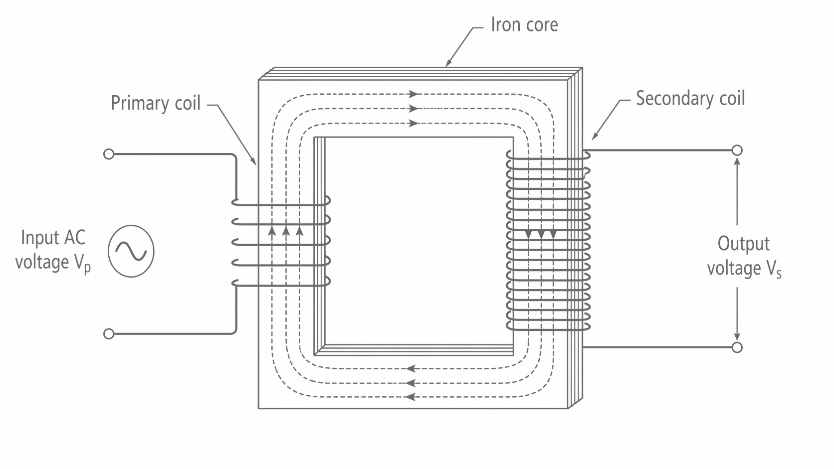
The core provides a low-reluctance path that links most of the flux through both coils. Current does not travel through the core from primary to secondary. A secondary emf exists even when its circuit is open; a load completes the secondary circuit so current and useful power can be supplied.

Changing core flux also induces a back emf in the primary, opposing the applied voltage. With the secondary open, the small primary current provides magnetisation and supplies core losses. When a load draws secondary current, its magnetic effect opposes the original change. The primary draws extra current to maintain approximately the same alternating core flux and to supply the load's power. Normal loading does not permanently eliminate the back emf.

Steady dc produces no sustained changing flux after the switch-on transient, so there is no sustained secondary output. The primary can then take excessive current limited largely by winding resistance. Transformer action requires changing flux; ordinary transformers are operated with ac, while a switched current can also produce changing flux.

Voltage ratio from Faraday’s law

If the same flux $\Phi$ links every turn of both coils, their induced emf magnitudes are proportional to their turn counts: $|\varepsilon_p|=N_p|\mathrm d\Phi/\mathrm dt|$ and $|\varepsilon_s|=N_s|\mathrm d\Phi/\mathrm dt|$. Dividing cancels the common flux-change rate.

For an ideal transformer the terminal voltages equal the induced emf magnitudes. The relation is a good approximation when winding voltage drops and flux leakage are small. Compare like measures: rms with rms, or peak with peak. A step-up transformer has $N_s>N_p$, while a step-down transformer has $N_s<N_p$. The frequency is unchanged.

For example, $N_p=1150$ and $V_p=230\,\mathrm V$ require $N_s=1150(12/230)=60$ turns for $12\,\mathrm V$. A turns ratio of $1:4$ multiplies voltage by four; it does not multiply power by four.

Investigating the ratio

Use an isolated low-voltage ac supply on the primary and ac voltmeters across the two windings. Keep the primary voltage, frequency and core assembly fixed, and change the number of secondary turns using taps. With a high-resistance voltmeter as the only secondary load, plot $V_s$ against $N_s$. A straight line through the origin has gradient $V_p/N_p$. Record the primary voltage for each reading rather than assuming the source is perfectly constant. This investigates the voltage ratio without confusing it with loaded winding losses.

Power, current ratio and efficiency

An ideal transformer conserves transferred power, so stepping up voltage reduces current for a given load power. In the school model used here, voltages and currents are rms and their phases allow mean power to be written as $IV$. A resistive secondary load and negligible magnetising current provide this approximation. If phase effects are significant, determine real input and output power directly rather than treating every rms product as real power.

For a real transformer, $I_sV_s=\eta I_pV_p$, not equal input and output power. If $\eta$ is stated as a percentage, divide by $100$ before using it as a factor. Power dissipated is $P_{\mathrm{in}}-P_{\mathrm{out}}$.

A transformer delivers $12\,\mathrm V$ at $4.0\,\mathrm A$, so output power is $48\,\mathrm W$. At $90\%$ efficiency, input power is $48/0.90=53.3\,\mathrm W$. With $230\,\mathrm V$ input, $I_p=53.3/230=0.232\,\mathrm A$; dissipated power is $5.33\,\mathrm W$. Multiplying output power by efficiency would wrongly make input smaller than output.

When investigating load current, place ammeters in series with the respective coils and voltmeters in parallel. Vary a suitable secondary load resistance, recording both currents and voltages. Avoid shorting a winding; respect the rated current and allow hot resistors to cool. For an approximately ideal transformer, $I_p/I_s$ should approach $N_s/N_p$ as load current becomes appreciable compared with the no-load current.