3.7.3.2 - Electric Field Strength

Reading field-line patterns

An electric field describes the force that source charges would exert on a stationary test charge placed at a point. The tangent to a field line gives the force direction on a positive test charge. Field lines are a representation, not material threads or compulsory particle paths.

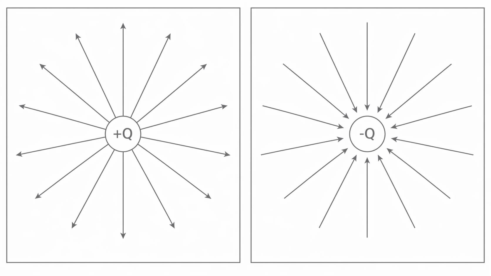
Lines point away from positive charges and towards negative charges, or extend to or from infinity. They never cross: crossing would assign two different directions to one field vector. More closely packed lines represent a stronger field when a consistent line convention is used. Lines meet conducting surfaces normally in electrostatic equilibrium; a tangential field would move the free surface charges.

[DIAGRAM: asset_name: 7.3.2 - Electric Field Strength - Diagram 1; asset_slug: 7.3.2 - Electric Field Strength - Diagram 1; caption: Radial fields point away from positive charge and towards negative charge; description: Isolated positive and negative charges produce radial patterns with opposite arrow directions.]

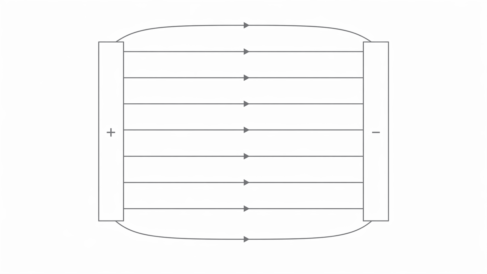
Between broad, oppositely charged parallel plates, the central field is approximately uniform: both its magnitude and direction are constant. Field lines are parallel, equally spaced and normal to the plates. Near an edge they bend and spread, so the uniform approximation fails there.

[DIAGRAM: asset_name: 7.3.2 - Electric Field Strength - Diagram 2; asset_slug: 7.3.2 - Electric Field Strength - Diagram 2; caption: The central field between plates is uniform and points from positive to negative; description: Parallel central field lines point from the positive plate at left to the negative plate at right. Curved outer lines indicate the non-uniform edge region schematically.]

Field strength and the sign of the test charge

Electric field strength is force per unit positive test charge at a point. The test charge must be small enough not to appreciably disturb the source distribution. The field belongs to the sources: changing the test charge changes the force, not the undisturbed field.

With signed $q$, these are vector equations. For magnitudes use $E=F/|q|$. A positive charge has force parallel to $\mathbf E$; a negative charge has force antiparallel. The unit is $\mathrm{N\,C^{-1}}$, also written $\mathrm{V\,m^{-1}}$.

A $-2.0\,\mathrm{nC}$ test charge experiences $6.0\,\mu\mathrm{N}$ west. Taking east positive, $E_x=(-6.0\times10^{-6})/(-2.0\times10^{-9})=+3.0\times10^3\,\mathrm{N\,C^{-1}}$: the field points east. A positive charge placed there would be forced east. A force direction alone cannot specify the field until the test-charge sign is known.

For several sources, add the fields as vectors first, then use $\mathbf F=q\mathbf E_\mathrm{resultant}$. For example, perpendicular components $E_x=300\,\mathrm{N\,C^{-1}}$ and $E_y=-400\,\mathrm{N\,C^{-1}}$ give $E=500\,\mathrm{N\,C^{-1}}$, directed $53.1^\circ$ below the positive horizontal axis. A negative particle is forced in the opposite direction.

Deriving the field between parallel plates

A potential difference is an energy change per unit charge. To derive the plate-field magnitude, define $U=V_\mathrm{high}-V_\mathrm{low}>0$ as the potential drop from the positive plate to the negative plate, separated by perpendicular distance $d$. This avoids confusing a positive drop with the signed final-minus-initial change in potential.

A positive charge $q$ moving along the field from high to low potential experiences constant force $F=qE$. The work done by the field is $W_\mathrm{field}=Fd$. Its potential energy falls by $qU$, so the field's positive work is $qU$. Therefore

This is the required $Fd=Q\Delta V$ magnitude relationship, with $\Delta V$ interpreted as the positive plate potential difference. If instead $\Delta V=V_\mathrm{final}-V_\mathrm{initial}=-U$, then $W_\mathrm{field}=-q\Delta V$.

The magnitude equation applies to the central region of parallel plates with negligible fringing. It does not give the local field around a point charge merely by dividing its potential by an arbitrary distance.

For plates $20\,\mathrm{mm}$ apart with $U=600\,\mathrm{V}$, $E=600/0.020=3.0\times10^4\,\mathrm{V\,m^{-1}}$. A particle of charge $-4.0\times10^{-19}\,\mathrm{C}$ experiences force magnitude $1.2\times10^{-14}\,\mathrm{N}$ towards the positive plate. Since $1\,\mathrm{V}=1\,\mathrm{J\,C^{-1}}$ and $1\,\mathrm{J}=1\,\mathrm{N\,m}$, $\mathrm{V\,m^{-1}}=\mathrm{N\,C^{-1}}$.