RP01 - Stationary Waves on a String
Investigate how the first-harmonic frequency depends separately on vibrating length, tension and mass per unit length. Recognise the mode, measure a repeatable resonance, analyse all the data and test the model with justified uncertainties.
Predicting the resonant frequencies
A vibration generator launches transverse waves along a stretched string. Reflection at a support sends waves back; their superposition gives a large, nearly stationary pattern near a resonant frequency. The ideal model has equal counter-propagating waves and fixed nodes. A real driver moves slightly and supplies energy lost through damping, so its effective node is approximate.
For the first harmonic, the vibrating length contains one half-wavelength: one loop, two end nodes and one central antinode. Therefore , and
First harmonic
Here is tension in newtons and is mass per unit length in . Greater tension gives a stronger restoring force; greater mass per metre gives more inertia. At fixed , quadrupling doubles , while quadrupling halves it. At fixed and , halving doubles .
The required practical investigates all three dependencies in separate runs. A change in frequency by itself is not enough: decide which quantity varied and which were controlled. Keep the harmonic number fixed, since the third harmonic has three times the first-harmonic frequency on the same string.
Finding and measuring a resonance
The vibrating length must be defined by the effective end positions of the oscillating section, not by the full piece of string or the distance to the hanging load.
[DIAGRAM: asset_name: RP 01 - Investigation into the Variation of the Frequency of Stationary Waves on a String - Diagram 1; asset_slug: RP 01 - Investigation into the Variation of the Frequency of Stationary Waves on a String - Diagram 1; recommended_method: retained_png; caption: A driven string with adjustable vibrating length and a suspended load; description: Side view of the apparatus. From left to right: a retort stand with clamp holds a vibration generator. A string is threaded through the hole in the vibration generator and tied to the stand. The string extends horizontally to the right, passing over a wooden bridge (a small triangular wedge resting on the bench), then continues to a pulley clamped at the edge of the bench. The string hangs vertically downward from the pulley with a mass hanger (100 g) attached. The vibrating section of the string is the horizontal portion between the vibration generator and the bridge — label this length as . The signal generator is connected to the vibration generator by two leads. A 2 kg counterweight sits on the base of the retort stand. Label all components.]
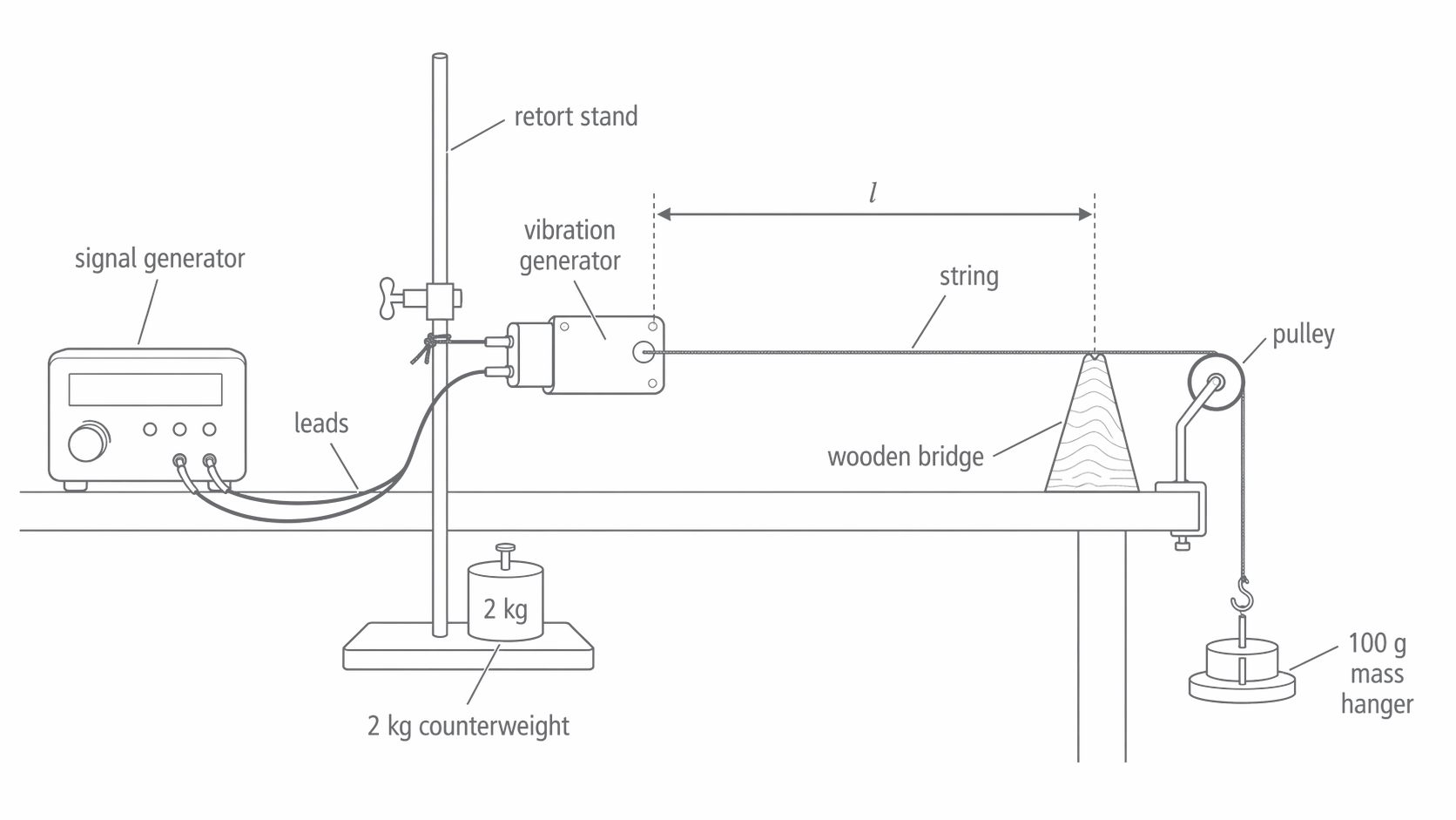
The bridge sets one end of the vibrating section. The string continues over the pulley to a freely hanging load; this continuation is not included in the vibrating length.
Connect a signal generator to a vibration generator supported by a firmly clamped or weighted stand. Pass the string through the driving attachment and over a bridge and a low-friction pulley to a load. Keep the vibrating section horizontal. The bridge constrains the string; the small driving motion approximates a node at the other end. Include the mass hanger in the total hanging mass , so while the load is stationary and friction is small.
Before assembly, measure the mass and length of a long sample of the same uniform string to obtain . A long sample gives a larger mass and lower percentage weighing uncertainty. The sample length used for is different from the vibrating length .
- Set and measure from the driving contact to the bridge. Read the ruler square-on; use a set square to transfer the contact positions to the scale.
- With modest driving amplitude, increase frequency slowly from below the expected first harmonic. Look for one loop. Tune through the peak amplitude from both directions and record the frequency.
- Repeat the tuning independently, rather than copying the display without changing anything. Use the spread and instrument information to estimate frequency uncertainty.
- Move the bridge to change over a broad measurable range, such as –. Repeat with the same string and hanging load. Record the actual lengths rather than only intended settings.
A lightweight paper rider near the antinode can help reveal large motion, but it can also load and damp a thin string. Direct observation or a suitable motion sensor can be preferable. Confirm the loop count rather than assuming the loudest response is the first harmonic. Allow electronic equipment to stabilise according to its instructions; an exact warm-up duration is not universal.
Clamp the apparatus securely, keep the load clear of feet with a tray below, and avoid excessive tension. For wire, use eye protection because a snapped wire may recoil. If a wire is driven by alternating current in a magnetic field, use the school's low-voltage isolated supply; never connect the wire directly to mains.
Separating length, tension and mass per length
Each investigation changes one physical variable. The controls follow from the equation, rather than from a memorised generic list.
| Changed quantity | Method | Controls | Straight-line graph | Predicted gradient |
|---|---|---|---|---|
| Move the bridge | Same load, same string, first harmonic | against | ||
| Change total hanging mass and use | Same measured , same string, first harmonic | against | ||
| Fit several strings; measure each sample's mass and length | Same measured , same load, first harmonic | against |
Squaring gives . This is directly proportional to when are fixed, and directly proportional to when are fixed. An equally valid length graph is against , whose gradient is .
For the tension run, recheck after changing the load: a stretchy string or moving support can alter the effective length and mass per unit length. For the run, compare uniform strings within a range where they remain flexible and nearly inextensible; changing a very stiff wire can make the simple string model less suitable. Record any failure of the controls, rather than assigning every discrepancy to random error.
Graphs that test the model
The AQA practical handbook gives the following length-run readings. The load is ; the sample string mass is over .
| 1.00 | 20.5 | 0.04878 | 41.0 |
| 0.90 | 23.5 | 0.04255 | 42.3 |
| 0.80 | 26.5 | 0.03774 | 42.4 |
| 0.70 | 30.0 | 0.03333 | 42.0 |
| 0.60 | 34.5 | 0.02899 | 41.4 |
| 0.50 | 42.0 | 0.02381 | 42.0 |
[DIAGRAM: asset_name: RP 01 - Investigation into the Variation of the Frequency of Stationary Waves on a String - Diagram 2; asset_slug: RP 01 - Investigation into the Variation of the Frequency of Stationary Waves on a String - Diagram 2; caption: Reciprocal frequency varies linearly with string length; description: Uniform-axis graph of reciprocal frequency against vibrating length using all six table readings. The unconstrained best-fit gradient is approximately 0.0486 seconds per metre. A large gradient triangle uses two points on the fitted line. Error bars use an explicitly assumed frequency uncertainty of 0.5 Hz. No worst-acceptable line is claimed.]
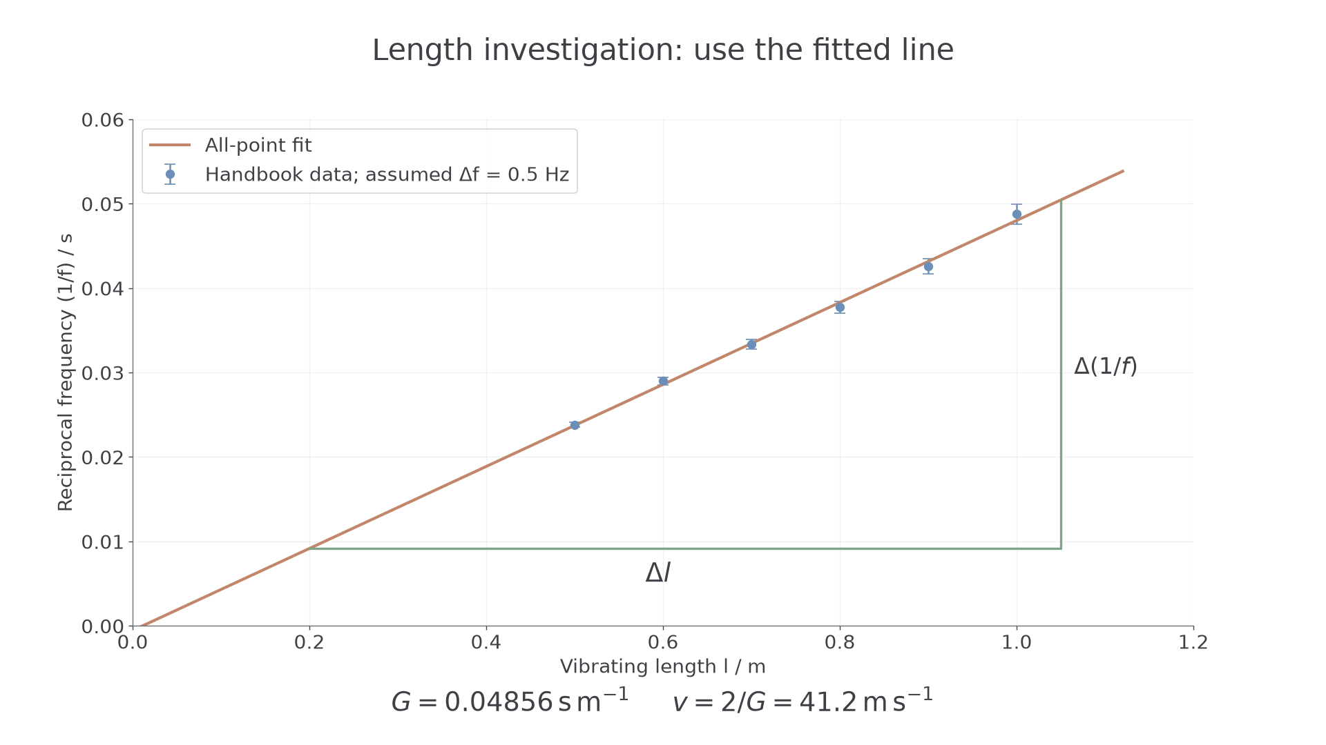
Exact plot of the handbook readings. The fitted line uses all six points; the triangle uses positions on that line. Error bars illustrate an assumed frequency uncertainty of ±0.5 Hz, not an uncertainty supplied with the original data.
Plot on the vertical axis and horizontally. The model predicts , so a straight line with intercept consistent with zero supports the inverse relationship. Fit the data before deciding whether forcing the line through zero is justified. A nonzero intercept can suggest a length offset, but scatter and uncertainty must be considered before declaring systematic error.
Calculate a gradient using widely separated points on the fitted line. Joining just the first and last data points is an endpoint estimate, not a best fit to all measurements. The string still contains one half-wavelength at each first-harmonic resonance: reducing reduces that wavelength; it does not reduce the number of half-wavelengths in the pattern.
For these readings an unconstrained least-squares line has gradient and intercept . Its wave-speed estimate is . A hand-drawn best fit may differ slightly. Report the method used rather than selecting endpoints to obtain a desired agreement.
Comparing measured and predicted speeds
A fitted trend and a physical prediction use different measurements. Comparing them is a test of the model only when their uncertainties and assumptions are visible.
From the handbook string measurements,
The all-point graph estimate, , differs from the prediction by approximately . That is a discrepancy, not an uncertainty. Decide whether it is significant by comparing justified uncertainty intervals; closeness alone does not establish accuracy.
For a single independent reading, suppose and . Then and . This gives a useful check but does not replace the graph. If the observed pattern actually had two loops, and the true speed would be half the first-harmonic calculation.
The same measurements can estimate tension: . This is how resonance can test the tension in a cable without removing it. Check the harmonic number and effective vibrating length before using that inference.
Uncertainty, offsets and improvements
Choose measurement uncertainties from instrument resolution, calibration information and the observed difficulty of the measurement. Repeated tuning may give a half-range larger than the display resolution. A tiny half-range does not remove instrument uncertainty or a systematic calibration error.
For , the factor two is exact. A conservative A-level estimate adds fractional uncertainties:
For and , the percentage uncertainty is . Thus . The length uncertainty here is given for the full measured separation. Do not automatically halve an instrument's quoted uncertainty.
For , add the mass and sample-length percentage uncertainties. For , halve the sum of the percentage uncertainties in and . For example, a sample measured with stated uncertainty has mass uncertainty . Using an unsuitable uncertainty would give about , so a longer sample or a suitable balance is a targeted improvement.
For the graph, convert frequency uncertainty into reciprocal-frequency error bars using for small fractional errors. Draw the steepest or shallowest acceptable line through the error bars. Estimate . Since , its percentage uncertainty is approximately the same as the gradient's. Do not draw a 'worst acceptable' line that misses the bars; if no line intersects them all, reconsider the uncertainty estimates or the straight-line model.
A constant length error has a characteristic sign. If the recorded length is smaller than the true effective length by , then : the intercept is positive. Repeating the same wrong reference point cannot fix it. Locate the effective end positions more carefully.
Pulley or bridge friction can make the vibrating-section tension differ from ; the direction depends on the loading history. A frequency calibration error can shift all frequency readings. Check the pulley freedom and generator frequency independently. Improve resonance detection when tuning uncertainty dominates, and improve weighing when uncertainty in dominates. An improvement should address the largest relevant contribution, not simply replace every instrument.