RP02 - Interference Effects
Use Young’s double slit and a normally illuminated transmission grating to measure laser wavelength. Choose measurable spans, convert screen geometry correctly and compare results using their uncertainties.
Connecting path difference to measurements
Both methods use normally incident laser light to produce coherent sources in phase. At a principal maximum the relevant path difference is a whole number of wavelengths. The double slit measures closely spaced fringes; the grating measures the directions of narrow principal maxima.
For the double slit, two narrow slits separated by diffract light into overlapping beams. Close to the centre of a distant screen,
Here is the distance from the slit plane to the screen and is the distance between adjacent bright centres or adjacent dark centres. The approximation requires nearly parallel outgoing paths () and a small observation angle (). Large alone does not guarantee a small angle far across the screen.
For a transmission grating at normal incidence,
Convert line density before taking its reciprocal: is . The angle is measured from the straight-through beam, which is normal to the grating. A maximum requires ; the finite screen can show fewer orders. An order at exactly does not meet a forward screen.
Coherence means constant phase difference, not merely equal wavelength. The laser feeds the slits coherently; equal amplitudes allow complete cancellation at dark fringes. The many grating slits give narrow maxima because a small angular change accumulates phase differences across the array, causing cancellation away from the principal directions.
Setting up the two experiments
Use a school-approved low-power laser, a securely mounted slide or transmission grating, a matt screen and rulers. The beam must be below everyone's eye level, end on a screen or beam stop, and never be viewed directly or along a reflection. Remove reflective objects from the beam area; switch off before rearranging the apparatus. Partial darkening aids visibility without making movement around the apparatus unsafe.
Young's double slit
[DIAGRAM: asset_name: RP 02 - Investigation of Interference Effects - Diagram 1; asset_slug: RP 02 - Investigation of Interference Effects - Diagram 1; caption: Young’s apparatus: measure spacing between adjacent bright fringes; description: Plan-view Young double slit geometry with coherent illumination, slit separation s, perpendicular screen distance D, and a magnified bright-fringe strip identifying adjacent-centre spacing w.]
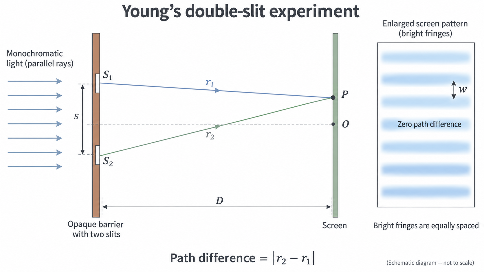
Measure D from the slit plane. The enlarged screen view defines w between adjacent bright centres; count intervals rather than counting bright lines.
- Illuminate both narrow slits evenly and align the screen perpendicular to the central beam. Record the calibrated centre-to-centre slit spacing . Use a travelling microscope or another suitable calibrated method if it must be measured; ordinary callipers are poorly suited to a spacing near .
- Set a measured , initially about . Mark centres of two clearly identifiable fringes separated by several intervals near the centre. Measure their span and count the intervals .
- Calculate . From the first to the eleventh bright centre there are ten intervals. Do not combine a bright centre and an adjacent dark centre as one full interval.
- Repeat the span measurement independently. Change over a useful range while retaining the same slide and laser; realign the screen at each position. Record actual , interval count and repeat spans.
Transmission grating
[DIAGRAM: asset_name: RP 02 - Investigation of Interference Effects - Diagram 2; asset_slug: RP 02 - Investigation of Interference Effects - Diagram 2; caption: Grating orders spread at unequal angles around the normal; description: Exact normal-incidence grating geometry. Rays reach the screen symmetrically in zero, first and second orders. Higher orders are not equally spaced. The perpendicular distance D and transverse height h2 define the angle triangle.]
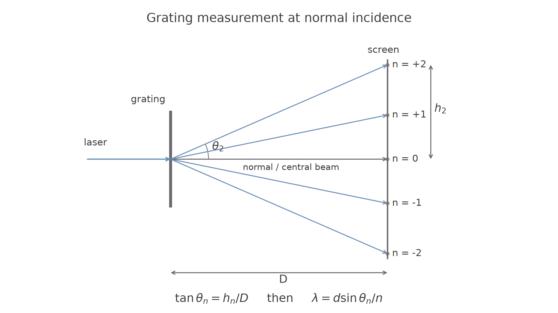
The normal is the horizontal straight-through direction. At normal incidence, corresponding positive and negative orders are symmetric; D and h form the angle triangle.
- Replace the slide by a plane transmission grating at normal incidence. Record its line density and calculate . Set and measure the perpendicular grating-to-screen distance .
- Mark the zero-order spot and corresponding positive and negative orders. Check symmetry; a large asymmetry means the alignment should be corrected before proceeding.
- For each order, measure the centre-to-centre separation between the two opposite spots. Then , reducing sensitivity to an uncertain zero-order mark. Alternatively measure each side from the centre and compare them.
- Calculate , then . Use several clear orders and independent repeats. Keep each result so disagreement can reveal misidentification or misalignment.
Averaging corresponding sides reduces centring errors and some effects of small misalignment; it does not make an obliquely illuminated grating obey the normal-incidence formula exactly. Align first. Do not replace by at large angles: that ratio is .
Choosing controls and a useful range
A good design produces measurable changes while keeping the model's other quantities fixed. More readings in a tiny range add little information about a gradient.
| Method | Varied or compared | Measured response | Main controls |
|---|---|---|---|
| Double slit | Screen distance | Fringe spacing | Same and laser wavelength; perpendicular screen; use central fringes |
| Grating | Order number | , hence | Same , wavelength, and normal incidence |
For the double slit, choose enough screen distances to establish a trend, for example six or more from to if the fringes remain clear. A larger increases the fringe span, reducing the fractional position-reading uncertainty, but may make the pattern too faint or too wide. Use as many intervals as can be counted confidently without leaving the small-angle central region.
For the grating, higher orders often give a larger measurable separation and lower fractional position uncertainty. They can also be faint or fall beyond the screen. Choose usable orders, not simply the largest theoretical order. Do not infer precision merely from the number of data points: slit or grating calibration can dominate every result.
If a repeated reading is anomalous, check the fringe count, order number, alignment and transcription; repeat it if possible. Exclude it only with a stated reason. Repeating the same setup does not remove a shared calibration error.
Extracting wavelength from a graph
The following double-slit readings are from the AQA practical handbook, with . The individual values need not lie exactly on the model line.
| 0.50 | 3.11 |
| 0.70 | 4.44 |
| 0.90 | 5.66 |
| 1.00 | 6.27 |
| 1.30 | 8.21 |
| 1.50 | 9.42 |
[DIAGRAM: asset_name: RP 02 - Investigation of Interference Effects - Diagram 3; asset_slug: RP 02 - Investigation of Interference Effects - Diagram 3; caption: The gradient of fringe spacing against screen distance gives wavelength divided by slit separation; description: Uniform-axis graph using all six measured pairs of screen distance and fringe separation. The unconstrained best-fit line has gradient 6.303 millimetres per metre. The triangle is drawn on the fitted line.]
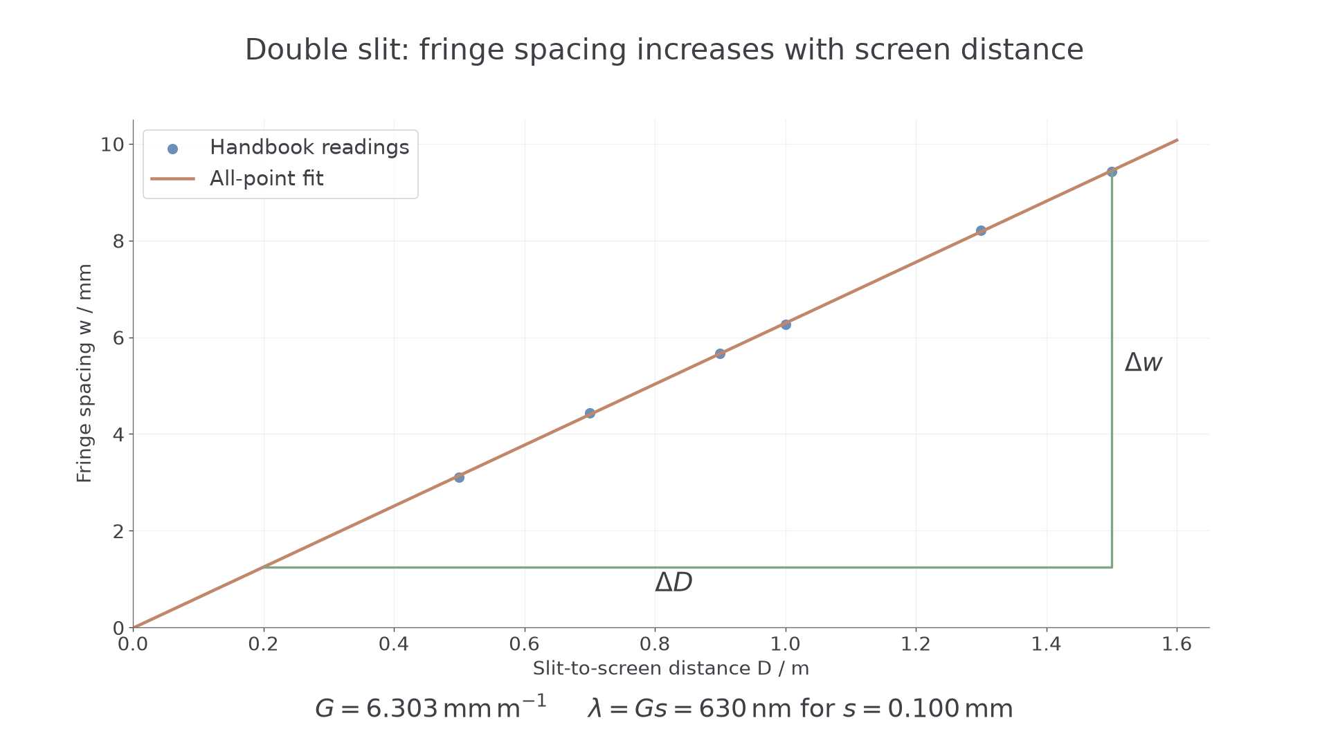
Exact plot of all six readings with a fitted line and a gradient triangle. The vertical values are millimetres, so the gradient must be converted before multiplying by s in metres.
From , the gradient of against equals when both distances use the same units. An unconstrained fit to all six readings gives and an intercept of . Thus
In SI units, and , giving
A hand-drawn line close to this trend is reasonable. Use a large triangle on that line, not simply two selected raw points. Test whether the intercept is consistent with zero within uncertainty. Do not force it to zero just because the ideal model predicts it.
A constant offset in recorded can give a nonzero intercept while leaving the gradient unchanged. A wrong slit spacing changes the inferred wavelength directly. These are different effects, so a nonzero intercept alone does not diagnose the slit spacing.
For the grating, plot against the exact integer . The model predicts gradient , so . The order number is exact only when correctly identified; miscounting an order is a mistake, not a tiny uncertainty. Fit all usable orders and examine the residual scatter.
Calculating the grating angle correctly
The screen measures a triangle, whereas the grating equation uses a sine. Keep these two steps distinct or use the exact combined expression
For the handbook example take and (100 lines per millimetre). The second-order displacement is :
Processing the four handbook displacements , , and with their respective orders 1–4 gives approximately , , and . Their mean is . Agreement between orders is encouraging, but a common error in would shift all of them together.
For a larger angle the distinction becomes substantial. If , the angle is , so , whereas . Treating the tangent as the sine would overestimate wavelength by about .
Uncertainty and experimental bias
State the uncertainty of the whole measured span before propagating it. Instrument resolution, manufacturer information and the difficulty of locating a fringe all matter. Repeats provide a spread; a small spread does not prove the span is known more precisely than the instrument permits.
Suppose ten intervals span . Then : division by the exact count changes absolute uncertainty but preserves percentage uncertainty, . With , a conservative percentage estimate adds those in , and .
If and , the wavelength percentage uncertainty is approximately . Improving a screen-distance contribution is less useful than calibrating the slit separation more accurately.
For the grating, propagate the measured geometry rather than assuming the fractional uncertainty in is automatically the fractional uncertainty in at every angle. A straightforward bound is to evaluate using the largest plausible and smallest plausible for an upper estimate, then the opposite limits for a lower estimate. In a graphical analysis use the best and worst acceptable gradients and include uncertainty in .
A ruler held away from the screen causes parallax; read square-on with the scale in the measurement plane. A tilted screen distorts the geometry. A grating tilted away from normal incidence invalidates the simple normal-incidence equation; persistent left–right asymmetry is a reason to realign. A wrongly quoted or produces a common scale bias which averaging cannot remove.
Comparing results with their uncertainties
A grating often gives narrower maxima and larger useful separations than a double slit, which can improve position measurement. It is not automatically the more accurate method: a poorly calibrated grating or a tilted setup can produce a precise but biased value.
Suppose the double slit gives and the grating gives . The intervals overlap, so the results are consistent within their stated uncertainties. The grating result is more precise because its uncertainty interval is narrower. Neither result alone proves the absence of systematic error.
If the two intervals do not overlap, investigate slit/grating calibration, units, order or fringe counts and alignment before choosing one result or averaging both. A mean of conflicting methods can conceal the problem. Comparing with a reference wavelength requires the reference's uncertainty too.
This comparison connects the full practical: coherent superposition creates the pattern, measured geometry determines wavelength, and an uncertainty analysis determines how strongly the evidence supports that value.