FS2 7.2 - The paired t-test
When observations belong together, analyse their differences together. You will recognise paired data, test a population mean difference and construct an interval for it, using the number of pairs and the spread of the differences.
The pair is the unit of comparison
If the mean of the differences equals the difference of the means, why bother keeping the pairs?
Because pairing changes the relevant spread. Six people complete a task before and after training:
| Person | A | B | C | D | E | F |
|---|---|---|---|---|---|---|
| Before, seconds | ||||||
| After, seconds |
Every person improves by between and seconds, despite the large differences between people's original completion times. Comparing each person with themselves retains that information.
You already know
For independent observations from one normal population with unknown variance, standardise their sample mean using their unbiased sample standard deviation and use . A confidence interval estimates a fixed population mean through a repeated-sampling rule.
The observations for one person are linked, so the two rows are not independent samples. Different people, or separately selected matched pairs, must provide independent differences.
Paired t-test
A paired t-test is a one-sample t-test on the differences within matched pairs. Define the difference direction consistently, for example , and test its population mean .
For the exact procedure, assume the differences between paired observations come from a normal population, with independent differences across pairs.
The normality assumption concerns differences. Separate assertions that both measurement rows look normal do not state the required condition. Equal variances in the two rows are not required, and independence within a pair is not required.
Before-and-after measurements on the same people are paired. Measurements on unrelated people randomly assigned to two separate groups are not automatically paired just because the group sizes match.
[DIAGRAM: asset_name: Wide individual times but small paired improvements; asset_slug: 9fm0-fs2-134-paired-changes; caption: Subtract within each person before estimating the spread of improvement; description: Six separate horizontal rows labelled A to F show grey segments joining each person's after and before completion times on a common seconds axis. After markers are pale blue and before markers pale clay, identified by a key. Each row has its positive before-minus-after difference, one,two,one,three,two,three, printed in a separate right column. A note gives six pairs and five degrees of freedom. The large variation in original times and small within-person changes are visible]
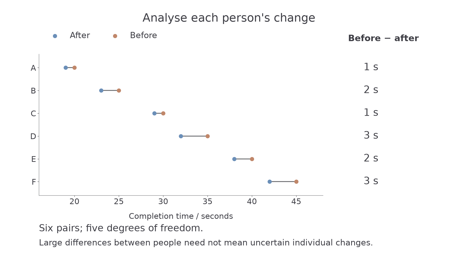
Here the correct difference variance is . If you wrongly reverse the after row before pairing it with the before row, the difference mean remains , but the difference variance becomes . The two marginal lists cannot recover the pairing information once it has been discarded.
Key idea
A paired analysis uses one sample of differences. Its sample size is the number of pairs, and its uncertainty comes from the differences' variation.
Choose the assumption that belongs to that one sample.
Test a claim about the mean difference
With , a positive value means a reduction in completion time. Write hypotheses in ; their direction follows this definition.
Paired t statistic
For independent differences from , with unknown , test using
Under , the statistic has degrees of freedom. These are the supplied one-sample variance and t formulas applied to matched-pair differences; the booklet explicitly includes matched pairs. In the formula booklet.
Calculate a signed difference for each matched pair before using a calculator's one-variable statistics. Subtracting the rows' sample standard deviations is not a method for finding .
Worked example 1: evidence of an improvement
Question. Use the six-person table to test at whether training is associated with a reduction in population mean completion time. Assume independent, normally distributed before-minus-after differences.
Plan. Form the differences, estimate their spread and use a positive one-tailed test.
Why this step? Positive before-minus-after differences mean improvement, so the claim belongs to the positive tail.
Answer. Reject . There is sufficient evidence at of a positive population mean reduction in completion time.
Check. There are six independent differences and therefore five degrees of freedom. The large statistic reflects consistent positive changes, rather than similarity in the original times.
Worked example 2 changes only the claimed threshold: the mean reduction must exceed , rather than .
Continue this lesson.
You’re previewing NovaLearn without an account. Create a free account to read the rest.
Create free account