D2 1.3 - Transportation as a linear program | Edexcel A-Level Further Mathematics

You will turn transportation tables into complete linear programs, define shipment variables with units, write source and destination constraints, and handle unused stock. You will also see why one balance equation is redundant in a balanced problem.

Give every route its own decision variable

Two depots supply three shops. There are two supply equations and three demand equations, yet one of those five equations is already forced by the other four. How can a condition be essential to describe the deliveries but add no new restriction?

We will answer that by turning a transportation table into a linear program. The table is a compact picture; the model spells out what each permitted plan must do.

You already know

From the north-west corner lesson, rows identify sources, columns identify destinations, and the margins give quantities. A linear program minimises or maximises a linear objective subject to linear constraints and specified variable domains. Define variables with units, state what is minimised, and translate each condition faithfully. A feasible plan satisfies every constraint; formulating a model does not require finding its optimum.

Suppose a divisible material is transported from depots A and B to shops P, Q and R. Every tonne held at the depots must be sent, and each shop must receive exactly its stated requirement.

Cost in pounds per tonne	P	Q	R	Supply, tonnes
A	$4$	$7$	$5$	$20$
B	$6$	$3$	$8$	$30$
Demand, tonnes	$10$	$15$	$25$

The entry $7$ is the cost of sending one tonne along route AQ. It is a fixed coefficient, not the quantity we choose to send.

Transportation decision variables

Let $x_{ij}$ be the number of tonnes transported from source $i$ to destination $j$ , where

i\in\{\mathrm A,\mathrm B\} \qquad j\in\{\mathrm P,\mathrm Q,\mathrm R\}

Thus $x_{\mathrm{AQ}}$ , for example, is the quantity sent from A to Q. All six variables are non-negative. They are continuous here because the material is divisible.

There is one variable for each permitted source–destination pair. A shop's requirement is not a decision variable: it is a fixed total that the chosen deliveries must meet. For indivisible crates, a model may instead require integer shipment quantities; choose the domain from what is transported.

Every shipment appears once in a source total and once in a destination total. That records its departure and arrival; it does not charge for the shipment twice.

[DIAGRAM: asset_name: One shipment belongs to two balance equations; asset_slug: 9fm0-d2-182-row-column-balances; caption: The AQ quantity appears in source A's row and destination Q's column.; description: A two-source three-destination table of shipment variables with supplies A20 B30 and demands P10 Q15 R25, highlighting the A row and Q column and displaying their separate balance equations.]

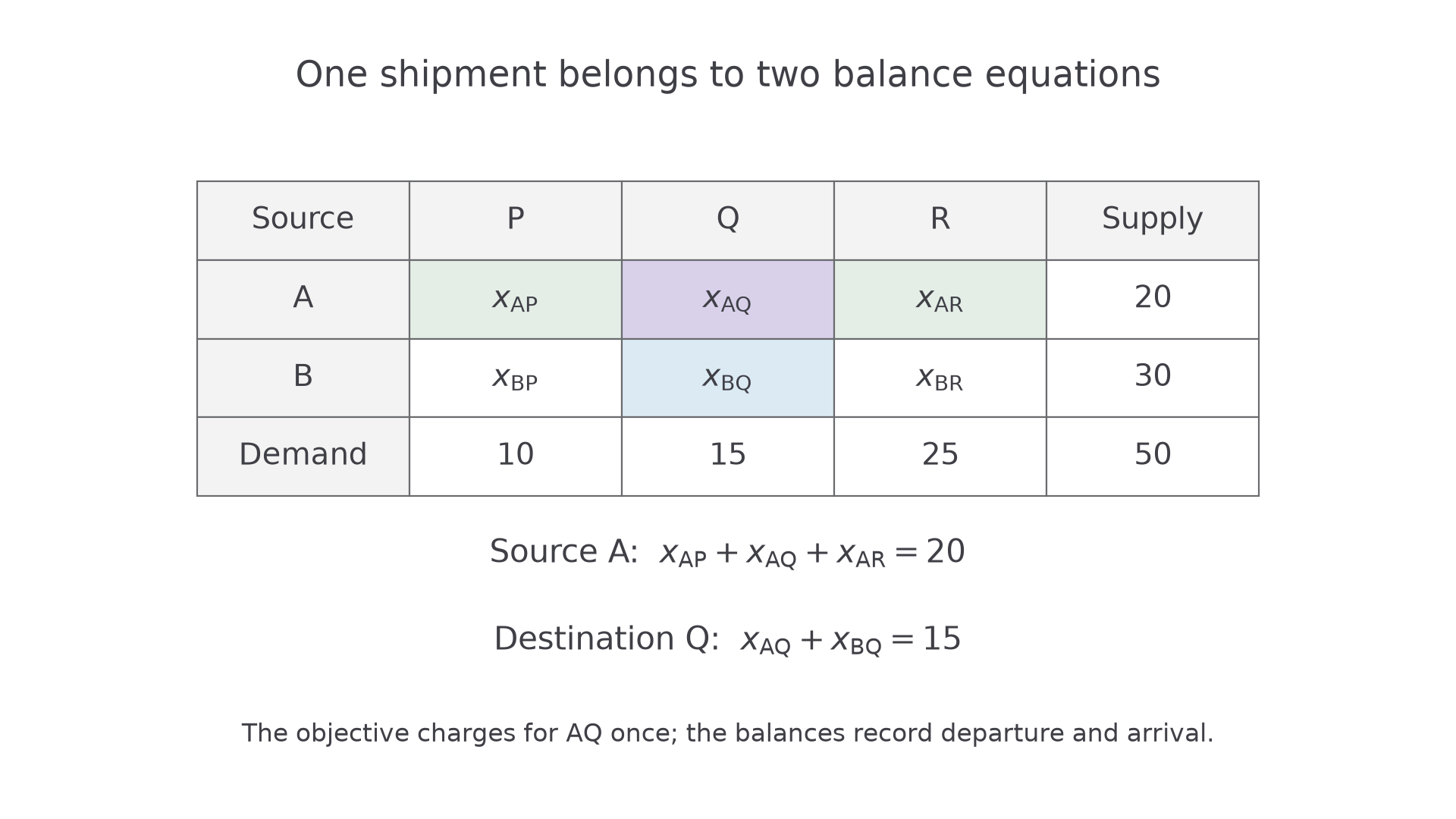
The objective charges $7x_{\mathrm{AQ}}$ pounds for route AQ once. In the constraints, $x_{\mathrm{AQ}}$ has coefficient $1$ , because one tonne leaving A is one tonne arriving at Q.

Key idea

Costs multiply shipment variables in the objective. Supply and demand constraints add shipment quantities with coefficient $1$ . State both index ranges so that every variable's route is unambiguous.

Check which expression actually totals the departures from A.

Write a complete balanced transportation model

Both margins total $50$ tonnes, so the table is balanced. Use a row equation for each source and a column equation for each destination.

For a general balanced table, let $s_i$ be source $i$ 's stock, $d_j$ destination $j$ 's exact demand, and $c_{ij}$ the unit transport cost. The following form assumes all stock is shipped and every demand is met exactly.

Balanced transportation linear program

With $m$ sources and $n$ destinations, and compatible quantity units,

\begin{aligned} \text{minimise }Z&=\sum_{i=1}^{m}\sum_{j=1}^{n}c_{ij}x_{ij}\\ \sum_{j=1}^{n}x_{ij}&=s_i &&(i=1,\ldots,m)\\ \sum_{i=1}^{m}x_{ij}&=d_j &&(j=1,\ldots,n)\\ x_{ij}&\ge0 &&(i=1,\ldots,m;\ j=1,\ldots,n) \end{aligned}

The margins must satisfy $\sum_i s_i=\sum_j d_j$ . Add integer restrictions if the transported units must be whole.

Not in the formula booklet: learn it.

Writing the model out in full is often the easiest way to check that no route or margin has disappeared. A double sum is equally valid when its coefficients and index ranges are clear.

Worked example 1: read each row and column

Question. Formulate the minimum-cost transportation problem for the table in the first part. Do not solve it.

Plan. Define the six shipment quantities, minimise the sum of unit cost times quantity, then impose the two source and three destination equations.

Let $x_{ij}$ be the tonnes transported from depot $i$ to shop $j$ , where $i\in\{\mathrm A,\mathrm B\}$ and $j\in\{\mathrm P,\mathrm Q,\mathrm R\}$ .

\begin{aligned} \text{minimise }Z={}&4x_{\mathrm{AP}}+7x_{\mathrm{AQ}}+5x_{\mathrm{AR}} +6x_{\mathrm{BP}}+3x_{\mathrm{BQ}}+8x_{\mathrm{BR}}\\ x_{\mathrm{AP}}+x_{\mathrm{AQ}}+x_{\mathrm{AR}}&=20 &&\text{stock at A}\\ x_{\mathrm{BP}}+x_{\mathrm{BQ}}+x_{\mathrm{BR}}&=30 &&\text{stock at B}\\ x_{\mathrm{AP}}+x_{\mathrm{BP}}&=10 &&\text{demand at P}\\ x_{\mathrm{AQ}}+x_{\mathrm{BQ}}&=15 &&\text{demand at Q}\\ x_{\mathrm{AR}}+x_{\mathrm{BR}}&=25 &&\text{demand at R}\\ x_{ij}&\ge0 &&\text{for every listed }i,j \end{aligned}

Why this step? Each column equation includes deliveries from both depots. Writing $x_{\mathrm{AP}}=10$ would unnecessarily force P to receive all its material from A.

Answer. The displayed minimisation, five balance equations and non-negative continuous domain form the model. $Z$ is the total transport cost in pounds.

Check. One feasible plan is

\begin{array}{c|rrr} &\mathrm P&\mathrm Q&\mathrm R\\\hline \mathrm A&10&10&0\\ \mathrm B&0&5&25 \end{array}

Its row totals are $20,30$ , its column totals are $10,15,25$ , and its cost is

4(10)+7(10)+3(5)+8(25)=325

This checks the meaning of the model; it does not establish that $325$ is the minimum.

Worked example 2 changes only the AQ unit cost, from $7$ to $9$ pounds per tonne. No quantity requirement changes.

Worked example 2: a new price changes the objective

Question. Formulate the revised model with AQ unit cost $9$ pounds per tonne.

Plan. Retain the shipment definitions and every balance equation. Replace only the coefficient of $x_{\mathrm{AQ}}$ .

Let $x_{ij}$ again be tonnes transported from $i$ to $j$ , with $i\in\{\mathrm A,\mathrm B\}$ and $j\in\{\mathrm P,\mathrm Q,\mathrm R\}$ . The complete model is

\begin{aligned} \text{minimise }Z={}&4x_{\mathrm{AP}}+9x_{\mathrm{AQ}}+5x_{\mathrm{AR}} +6x_{\mathrm{BP}}+3x_{\mathrm{BQ}}+8x_{\mathrm{BR}}\\ x_{\mathrm{AP}}+x_{\mathrm{AQ}}+x_{\mathrm{AR}}&=20\\ x_{\mathrm{BP}}+x_{\mathrm{BQ}}+x_{\mathrm{BR}}&=30\\ x_{\mathrm{AP}}+x_{\mathrm{BP}}&=10\\ x_{\mathrm{AQ}}+x_{\mathrm{BQ}}&=15\\ x_{\mathrm{AR}}+x_{\mathrm{BR}}&=25\\ x_{ij}&\ge0\quad\text{for every listed }i,j \end{aligned}

Why this step? A price change affects how attractive a plan is. It does not change which plans satisfy the stock and demand conditions.

Answer. Minimise the revised objective over the same feasible set.

Check. The earlier feasible plan still satisfies all five balance equations. It sends $10$ tonnes along AQ, so its cost rises by $2(10)=20$ , from $325$ to $345$ pounds.

Here is the promised surprise about the five equations. Add the two row equations: total deliveries are $20+30=50$ . If P receives $10$ and Q receives $15$ , R must receive $50-10-15=25$ . Its equation follows from the other four. This is why balanced transportation equations contain a redundancy, rather than five independent restrictions.

That observation does not license a mismatched margin. If R instead required $26$ tonnes while the other margins stayed fixed, exact total demand would be $51$ against stock $50$ , and the model would be infeasible. Present the full requested constraints clearly in a formulation answer.

Watch out

Wrong: omit “minimise”, leave the index ranges undefined, or multiply a balance equation by route costs. Right: define quantities and their routes, minimise total cost, and add unweighted quantities in every source and destination constraint.

Change the same unit cost once more; the logistics remain fixed.

Continue this lesson.

You’re previewing NovaLearn without an account. Create a free account to read the rest.

Create free account

Last Accessed

Core Pure Mathematics

Further Pure Mathematics 1

Further Pure Mathematics 2

Further Statistics 1

Further Statistics 2

Further Mechanics 1

Further Mechanics 2

Decision Mathematics 1

Decision Mathematics 2

D2 1.3 - Transportation as a linear program

Give every route its own decision variable

Write a complete balanced transportation model

Continue this lesson.

Learn faster with Nova