CP 7.2 - Sketching polar curves | Edexcel A-Level Further Mathematics

Sketch the standard polar curve families by combining admissible angles, symmetry and carefully chosen radius values. You will distinguish lines, circles, spirals, cardioids, dimpled curves and two different kinds of paired loops, using non-negative radius throughout.

A secant equation can represent a line

Which equation gives a straight line: $r=2\sec\theta$ or $r=2$ ? The first does; the second is a circle. A polar equation describes how distance changes as direction changes, so its appearance can be misleading.

You already know

Polar radius is distance, so $r\ge0$ . Use $x=r\cos\theta$ , $y=r\sin\theta$ , with angles measured from the initial line. A sketch should label the pole, the initial line and the important intercepts.

For positive $p$ , multiply $r=p\sec(\alpha-\theta)$ by $\cos(\alpha-\theta)$ . The compound-angle identity gives $r\cos\alpha\cos\theta+r\sin\alpha\sin\theta=p$ .

Straight lines in polar form

For $p>0$ ,

r=p\sec(\alpha-\theta) \quad\Longleftrightarrow\quad x\cos\alpha+y\sin\alpha=p

Use angles with $\cos(\alpha-\theta)>0$ , so the radius is positive. The line is perpendicular to the direction $\alpha$ , at distance $p$ from the pole.

Not in the formula booklet: learn it.

As a ray becomes nearly parallel to the line, its point of intersection moves arbitrarily far away. This explains an unbounded radius without an extra curved branch.

[DIAGRAM: asset_name: Two secant equations representing straight lines; asset_slug: 9fm0-cp46-lines; caption: A secant polar equation gives a straight line at a fixed perpendicular distance from the pole; description: Two equal-scale panels show x equals 2 from r equals 2 sec theta and x plus root 3 y equals 4 from r equals 2 sec pi over 3 minus theta. Each has pole and initial line marked, a normal from the pole of length 2, and the relevant axis intercepts.]
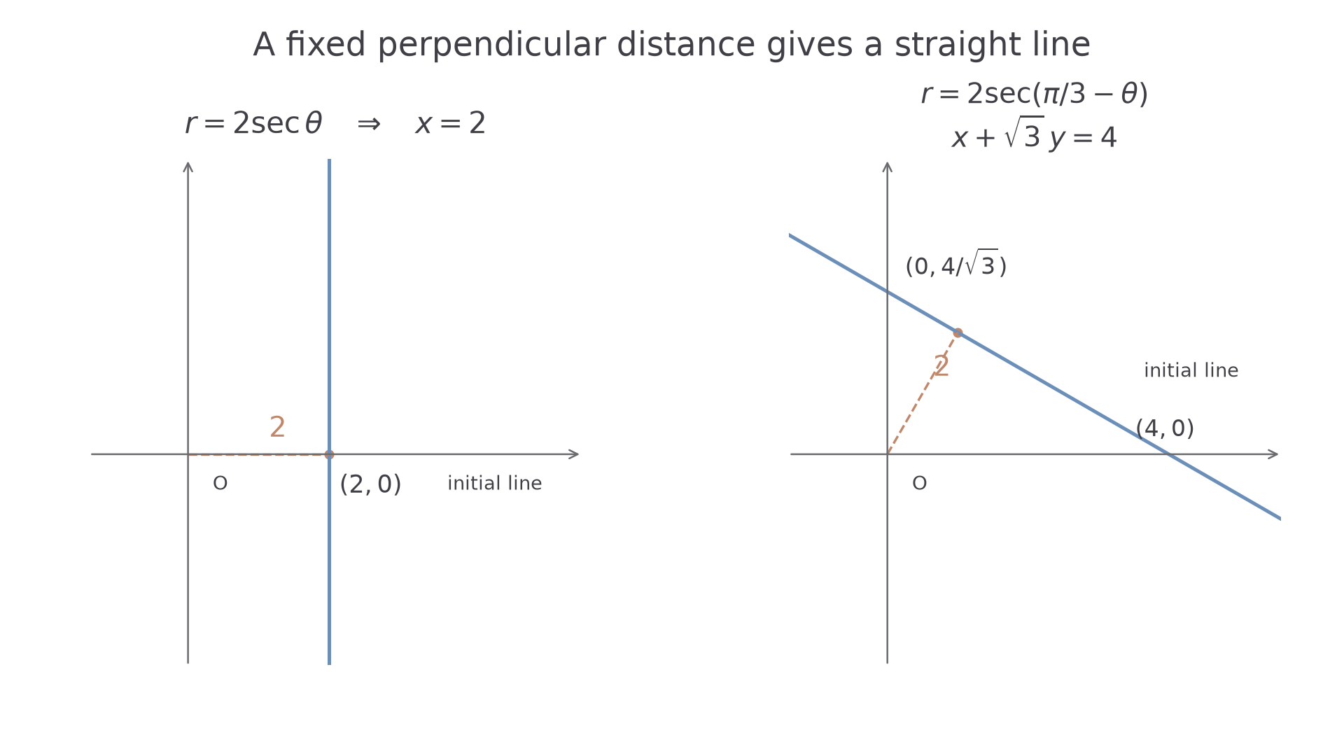
A secant polar equation gives a straight line at a fixed perpendicular distance from the pole

Worked example 1: a vertical line

Question. Describe and sketch $r=2\sec\theta$ .

Plan. Convert to Cartesian form, then find the admissible directions.

\begin{aligned} r\cos\theta&=2 && \text{multiply by cosine} \\ x&=2 && \text{Cartesian component} \\ -\frac\pi2<\theta<\frac\pi2 &&& \text{one complete admissible interval} \end{aligned}

Why this step? Positive cosine ensures positive radius. The excluded endpoint rays are parallel to the line and never meet it.

Answer. A vertical line through $(2,0)$ , two units to the right of the pole, as in the left panel.

Check. At $\theta=\frac\pi3$ , $r=4$ , giving $x=4\cos\frac\pi3=2$ .

Change only $\alpha$ , from zero to $\frac\pi3$ . The perpendicular distance stays $2$ , while the normal direction rotates.

Worked example 2: a rotated line

Question. Describe and sketch $r=2\sec(\frac\pi3-\theta)$ .

Plan. Expand the cosine after multiplying through, then find intercepts.

\begin{aligned} r\cos(\tfrac\pi3-\theta)&=2 && \text{remove secant} \\ \frac{x}{2}+\frac{\sqrt3\,y}{2}&=2 && \text{compound angle} \\ x+\sqrt3\,y&=4 && \text{Cartesian line} \end{aligned}

Why this step? The normal points at $\frac\pi3$ ; that is not the direction of the line itself.

Answer. The line joins intercepts $(4,0)$ and $(0,\frac4{\sqrt3})$ , with admissible directions $-\frac\pi6<\theta<\frac{5\pi}6$ , up to complete turns.

Check. At $\theta=\frac\pi3$ , $r=2$ , so $(x,y)=(1,\sqrt3)$ satisfies $x+\sqrt3\,y=4$ .

An asymptote of the secant function as a function of angle is not a second line on the Cartesian sketch.

Watch out

Wrong: plot radius vertically against angle and call that the polar curve. Right: each value of $r$ is a distance along its ray. The resulting locus here is a straight line.

Use the same normal-direction method after a further rotation.

Constant-radius circles and circles through the pole

A constant equation $r=a$ , with $a>0$ , is a circle centred at the pole, of radius $a$ . One complete turn traces it once. In contrast, $r=2a\cos\theta$ is a circle touching the pole, with centre $(a,0)$ and radius $a$ .

Multiplication by $r$ shows why: $r^2=2ar\cos\theta$ , so $(x-a)^2+y^2=a^2$ . Its non-negative-radius description uses $-\frac\pi2\le\theta\le\frac\pi2$ ; the endpoints both give the pole. These circle forms are not printed in the formula booklet.

[DIAGRAM: asset_name: A circle centred at the pole compared with one through the pole; asset_slug: 9fm0-cp46-circles; caption: The same circle radius can come from two different polar equations; description: Equal-scale panels show r equals 2 as a circle centred at the pole with radius 2 and r equals 4 cos theta as a circle centred at (2,0) with radius 2. The second passes through the pole and (4,0), and its admissible angular interval is minus pi over 2 to pi over 2.]
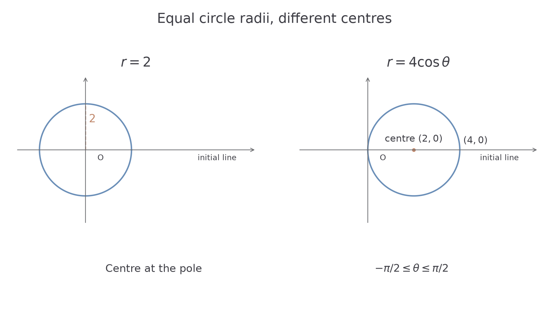
The same circle radius can come from two different polar equations

Worked example 3: a circle through the pole

Question. Describe the complete sketch of $r=4\cos\theta$ , with non-negative radius.

Plan. Identify the circle and the angles needed to trace it once.

\begin{aligned} r^2&=4r\cos\theta && \text{multiply by radius} \\ (x-2)^2+y^2&=4 && \text{complete the square} \\ -\frac\pi2\le\theta\le\frac\pi2 &&& \cos\theta\ge0 \end{aligned}

Why this step? The circle's radius is half its largest polar radius: the pole is on its edge, not at its centre.

Answer. Centre $(2,0)$ , radius $2$ , horizontal intercepts $O$ and $(4,0)$ , symmetric about the initial line.

Check. At $\theta=\frac\pi4$ , $r=2\sqrt2$ , giving $(2,2)$ , the top of the circle.

Change only the coefficient from $4$ to $8$ . Every distance doubles, while the admissible angles stay the same.

Worked example 4: scaling the circle

Question. Describe the complete sketch of $r=8\cos\theta$ .

Plan. Use the same circle conversion with the larger coefficient.

\begin{aligned} x^2+y^2&=8x && \text{multiply by }r\text{ and substitute} \\ (x-4)^2+y^2&=16 && \text{complete the square} \end{aligned}

Why this step? Scaling the polar radius scales both Cartesian components by the same factor, so the entire shape enlarges about the pole.

Answer. Centre $(4,0)$ , radius $4$ , horizontal intercepts $O$ and $(8,0)$ , using $-\frac\pi2\le\theta\le\frac\pi2$ .

Check. At $\theta=\frac\pi4$ , the point is $(4,4)$ , four units above the centre.

Replacing cosine by sine rotates this family through $\frac\pi2$ , giving centre $(0,a)$ and admissible angles $0\le\theta\le\pi$ .

Watch out

Wrong: draw $r=4\cos\theta$ as a circle of radius $4$ centred at the pole. Right: its greatest distance from the pole is $4$ , but its circle radius is $2$ .

Distinguish the fixed-radius circle from the touching circle explicitly.

A radius growing with angle gives a spiral

For $r=k\theta$ , with $k>0$ , non-negative radius requires $\theta\ge0$ . As the angle increases, the point turns anticlockwise and moves steadily away from the pole. A finite angle interval gives a finite piece of the spiral.

After one additional turn, the radius increases by $k(\theta+2\pi)-k\theta=2\pi k$ . Thus successive turns have exactly the same radial separation along any fixed ray. This constant spacing is a useful and surprising feature of the spiral.

[DIAGRAM: asset_name: An Archimedean spiral over two turns; asset_slug: 9fm0-cp46-spiral; caption: A full turn adds a fixed amount to the radius; description: Equal-scale axes show r equals theta from zero to four pi as an anticlockwise spiral starting at the pole. Its positive-horizontal-ray crossings have radii two pi and four pi, and a bracket between them is labelled radial gap two pi.]

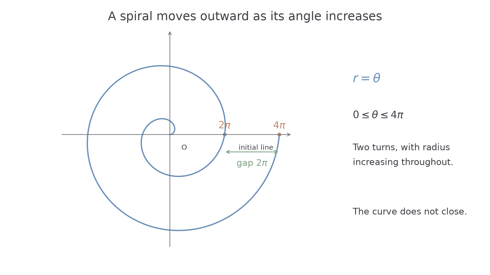
Worked example 5: one turn of a spiral

Question. Describe the sketch of $r=\theta$ for $0\le\theta\le2\pi$ .

Plan. Locate the pole, the quarter-turn points and the endpoint, then join in increasing angle order.

\begin{array}{c|ccccc} \theta&0&\pi/2&\pi&3\pi/2&2\pi\\\hline r&0&\pi/2&\pi&3\pi/2&2\pi \end{array}

Why this step? The radii grow while the rays rotate. Joining these points as a closed curve would ignore the unequal starting and finishing radii.

Answer. One anticlockwise turn, starting at the pole and ending at $(2\pi,0)$ , with continuously increasing radius.

Check. The endpoint lies on the initial line after one full turn; it is not back at the pole.

Change only $k$ , from $1$ to $2$ . The angular sweep is unchanged and each distance doubles.

Worked example 6: a more widely spaced spiral

Question. Describe $r=2\theta$ for $0\le\theta\le2\pi$ .

Plan. Double the previous radii at the same key angles.

\begin{array}{c|ccccc} \theta&0&\pi/2&\pi&3\pi/2&2\pi\\\hline r&0&\pi&2\pi&3\pi&4\pi \end{array}

Why this step? Changing $k$ changes scale, not the number of turns in a fixed angle interval.

Answer. One anticlockwise turn from the pole to $(4\pi,0)$ . If continued, successive turns have radial separation $4\pi$ .

Check. At $\theta=\pi$ , the point is $(-2\pi,0)$ , consistent with a positive radius on the leftward ray.

The spiral equation and its spacing result are not in the formula booklet. The equation itself makes the spacing easy to reconstruct.

Watch out

Wrong: $r(\theta+2\pi)=r(\theta)$ for this spiral because the rays agree. Right: the directions agree but the distances differ by $2\pi k$ .

Read a radius and a spacing directly from the next equation.

Cardioids have a cusp at the pole

The equations $r=a(1+\cos\theta)$ and $r=a(1-\cos\theta)$ , for $a>0$ , give cardioids. Their radii never become negative. Each has a cusp at the pole and is symmetric about the initial line, because cosine is unchanged when $\theta$ is replaced by $-\theta$ .

The plus form reaches its greatest radius $2a$ at $\theta=0$ and the pole at $\theta=\pi$ . The minus form reverses those directions. These shapes and their key values are not printed in the formula booklet.

[DIAGRAM: asset_name: Two reflected cardioids; asset_slug: 9fm0-cp46-cardioids; caption: Changing the cosine sign reflects the cardioid across the vertical axis; description: Separate equal-scale panels show r equals 2 times one plus cos theta opening right and r equals 2 times one minus cos theta opening left. Each has a cusp at the pole, vertical-axis intercepts at plus and minus 2, and its far horizontal intercept at plus 4 or minus 4.]
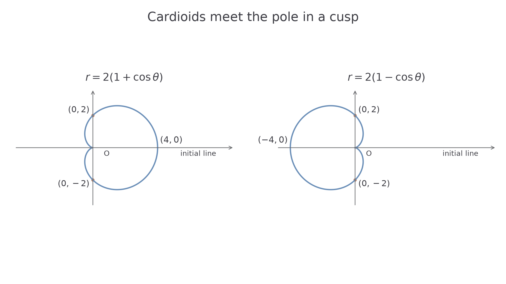
Changing the cosine sign reflects the cardioid across the vertical axis

Worked example 7: a right-facing cardioid

Question. Describe the sketch of $r=2(1+\cos\theta)$ , $0\le\theta\le2\pi$ .

Plan. Find the pole, maximum radius and axis points, then use symmetry.

\begin{array}{c|ccccc} \theta&0&\pi/2&\pi&3\pi/2&2\pi\\\hline r&4&2&0&2&4 \end{array}

Why this step? The zero at $\theta=\pi$ is a cusp at the pole; it is not a point two units to the left of the pole.

Answer. A right-facing cardioid through $(4,0)$ , $(0,2)$ , the pole and $(0,-2)$ , symmetric about the initial line.

Check. Since $-1\le\cos\theta\le1$ , the radius stays between $0$ and $4$ , as the sketch requires.

Change only the sign before cosine. The far point and the direction giving the pole swap sides.

Worked example 8: a left-facing cardioid

Question. Describe $r=2(1-\cos\theta)$ , $0\le\theta\le2\pi$ .

Plan. Use the same key angles with the changed sign.

\begin{array}{c|ccccc} \theta&0&\pi/2&\pi&3\pi/2&2\pi\\\hline r&0&2&4&2&0 \end{array}

Why this step? A positive radius at $\theta=\pi$ points left, so $r=4$ there gives $(-4,0)$ .

Answer. A left-facing cardioid with cusp at the pole, far horizontal point $(-4,0)$ , and vertical intercepts $(0,\pm2)$ .

Check. Replacing $\theta$ by $\pi-\theta$ turns the plus equation into the minus equation, confirming the reflection.

Replacing cosine by sine gives the same family turned through a right angle. Follow the actual equation to choose the orientation.

Watch out

Wrong: place the cusp at the smallest-looking horizontal intercept away from the pole. A cardioid's cusp occurs where $r=0$ , so it is the pole itself.

Change the scale while retaining the left-facing orientation.

A dimpled curve that misses the pole

For $r=a(3+2\cos\theta)$ , $a>0$ , the radius lies between $a$ and $5a$ . The curve has a small inward dimple near the negative horizontal axis and is symmetric about the initial line. It never reaches the pole, because its minimum radius is positive.

This is a dimpled limaçon. An axis point with minimum radius is not necessarily the leftmost point: distance from the pole and horizontal coordinate are different quantities. Use the full curve shape as well as its four axis points. This family is not printed in the formula booklet.

[DIAGRAM: asset_name: A dimpled limacon with positive minimum radius; asset_slug: 9fm0-cp46-limacon; caption: The minimum radius is positive and the left side has a dimple; description: Equal-scale axes show r equals 3 plus 2 cos theta. Axis points are (5,0), (0,3), (minus 1,0), and (0,minus 3). The curve has a visible left dimple and does not pass through the pole. The pole is marked separately inside the curve.]
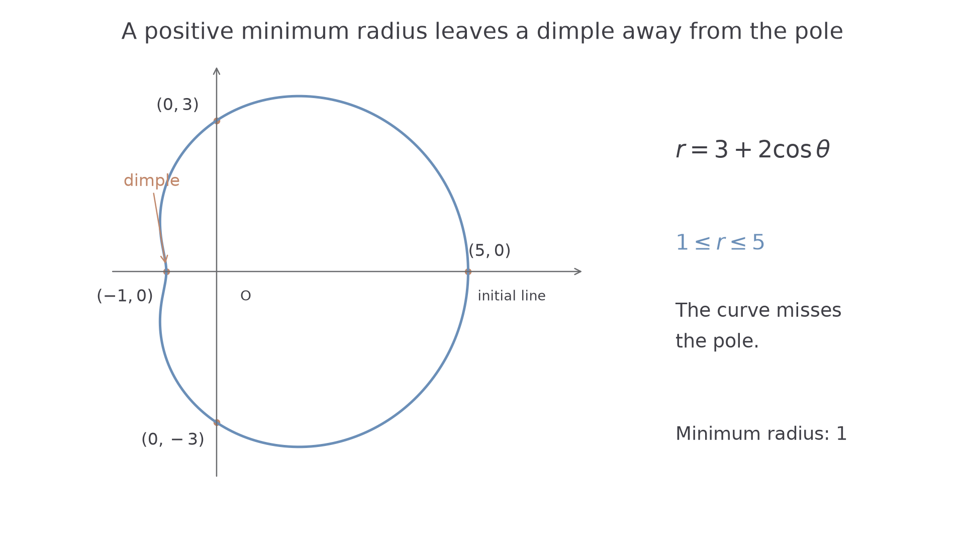
The minimum radius is positive and the left side has a dimple

Worked example 9: locating the dimple

Question. Describe the sketch of $r=3+2\cos\theta$ , $0\le\theta\le2\pi$ .

Plan. Bound the radius and locate the axis points, retaining the inward dimple.

\begin{array}{c|ccccc} \theta&0&\pi/2&\pi&3\pi/2&2\pi\\\hline r&5&3&1&3&5 \end{array}

Why this step? The value $r=1$ at $\theta=\pi$ gives $(-1,0)$ , so the curve misses the pole even on its closest ray.

Answer. A closed right-biased dimpled curve, symmetric above and below the initial line, through the four labelled axis points in the diagram.

Check. $3+2\cos\theta\ge1$ , so a sketch crossing the pole would contradict the equation.

Change only the scale factor from $a=1$ to $a=2$ . The dimple and symmetry remain; every distance doubles.

Worked example 10: scaling a dimpled curve

Question. Give the key sketch features of $r=2(3+2\cos\theta)$ .

Plan. Multiply each radius in the previous table by $2$ .

\begin{array}{c|cccc} \theta&0&\pi/2&\pi&3\pi/2\\\hline r&10&6&2&6 \end{array}

Why this step? An enlargement preserves whether the curve has a dimple and whether it passes through the pole.

Answer. Minimum radius $2$ , maximum radius $10$ , axis points $(10,0)$ , $(0,\pm6)$ , $(-2,0)$ ; the same dimpled shape and initial-line symmetry.

Check. At $\theta=\pi$ , the equation gives $2(3-2)=2>0$ , confirming that the pole is excluded.

The known dimple is a shape feature worth showing; four axis points joined as an ellipse would lose it.

Watch out

Wrong: call this a cardioid and put its cusp at the pole. Right: its minimum radius is $a>0$ ; draw a dimple away from the pole, with no cusp at the pole.

Extract the corresponding values at the next scale.

Double-angle cosine with non-negative radius

For $r=a\cos2\theta$ , $a>0$ , keep only angles for which $\cos2\theta\ge0$ . Under the distance convention $r\ge0$ , the complete curve has two horizontal loops. A plotting system that permits signed radius may add vertical lobes; those belong to a different coordinate convention.

One complete right loop is traced on $-\frac\pi4\le\theta\le\frac\pi4$ ; one complete left loop on $\frac{3\pi}4\le\theta\le\frac{5\pi}4$ . The curve is symmetric about both coordinate axes. Its maximum radius is $a$ , at $\theta=0$ and $\theta=\pi$ . This family is not printed in the formula booklet.

[DIAGRAM: asset_name: Admissible loops of r equals 2 cos 2theta; asset_slug: 9fm0-cp46-cosine-loops; caption: Non-negative radius gives two horizontal loops; description: Equal-scale axes show the right and left loops of r equals 2 cos 2theta, using only angles with cos 2theta non-negative. The tips are (2,0) and (minus 2,0). Dashed rays at pi over 4 and minus pi over 4 bound the right loop; the full admissible intervals for the two loops appear in a side panel. No vertical lobes are drawn.]
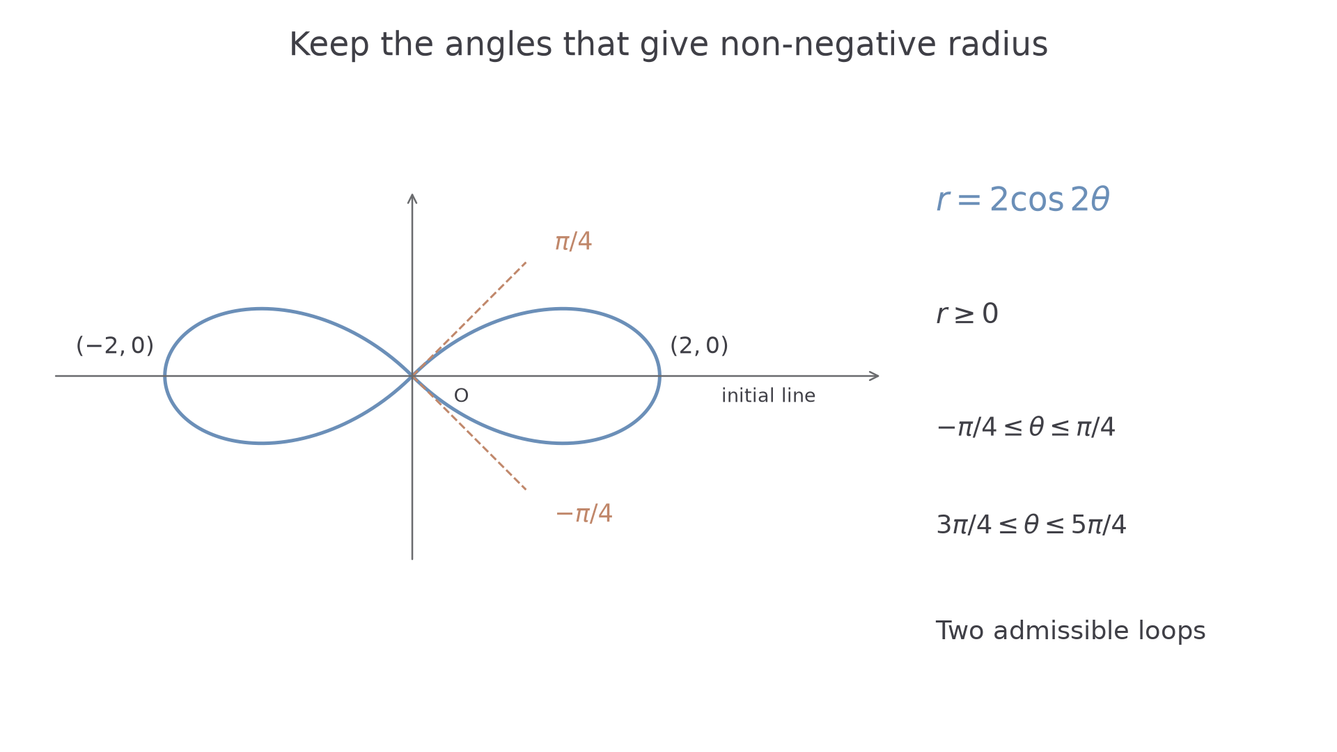
Non-negative radius gives two horizontal loops

Worked example 11: one pair of horizontal loops

Question. Give the key sketch features of $r=2\cos2\theta$ , with $r\ge0$ .

Plan. Solve $r=0$ , find the radial maxima and use the admissible intervals to trace the loops.

\begin{aligned} r=0&\Longleftrightarrow\cos2\theta=0 && \text{pole directions} \\ \theta&=\frac\pi4+\frac{k\pi}{2},\quad k\in\mathbb Z && \text{solve cosine zero} \\ r(0)&=r(\pi)=2 && \text{loop tips} \\ r(\pi/6)&=1 && \cos(\pi/3)=1/2 \end{aligned}

Why this step? Between $\frac\pi4$ and $\frac{3\pi}4$ , the formula would give a negative radius, so that interval contributes no points in this convention.

Answer. Two horizontal loops meeting at the pole, with tips $(\pm2,0)$ , traced on the two intervals stated above.

Check. At $\theta=\frac\pi2$ , the expression is $-2$ , so no point on the positive vertical ray is allowed.

Change only the coefficient from $2$ to $4$ . The admissible angles and loop directions remain the same.

Worked example 12: enlarging the two loops

Question. Describe $r=4\cos2\theta$ , with $r\ge0$ .

Plan. Keep the same pole directions and double the admissible radii.

\begin{aligned} r(0)&=r(\pi)=4 && \text{new tips} \\ r(\pi/6)&=2 && \text{double the previous radius} \\ r(\pi/4)&=0 && \text{same pole direction} \end{aligned}

Why this step? A positive scale factor does not change the sign of $\cos2\theta$ , so it cannot create new admissible angular intervals.

Answer. The same two horizontal loops enlarged by factor $2$ , with tips $(\pm4,0)$ .

Check. At $\theta=\frac\pi6$ , $(x,y)=(\sqrt3,1)$ , which lies in the upper half of the right loop.

Write the permitted intervals beside a sketch whenever part of the angular range is excluded.

Watch out

Wrong: replace a negative computed radius by its absolute value and keep the same angle. That plots a point which does not satisfy the equation. Right: exclude angles giving negative $r$ under the distance convention.

Use an intermediate scale to check the same structural features.

A squared-radius equation gives a lemniscate

The equation $r^2=a^2\cos2\theta$ , with $a>0$ , also needs $\cos2\theta\ge0$ , because $r^2\ge0$ . Taking the non-negative square root gives $r=a\sqrt{\cos2\theta}$ . Its two horizontal loops form a lemniscate.

The admissible intervals and the tip radii match those of $r=a\cos2\theta$ , but the curves are different between the pole and each tip. When $0<\cos2\theta<1$ , its square root is larger than the value itself. Thus the lemniscate extends farther out along each intermediate ray. Neither family is printed in the formula booklet.

[DIAGRAM: asset_name: Comparing a lemniscate with the cosine loops; asset_slug: 9fm0-cp46-lemniscate; caption: Equal tip radii and pole directions do not determine the whole curve; description: Equal-scale axes overlay blue r squared equals 4 cos 2theta and dashed clay r equals 2 cos 2theta, both restricted to non-negative radius. Both have tips at plus and minus 2 and meet at the pole. On the ray theta equals pi over 6, points mark radius root 2 on the lemniscate and radius 1 on the cosine loop. A legend sits outside the plotted curves.]
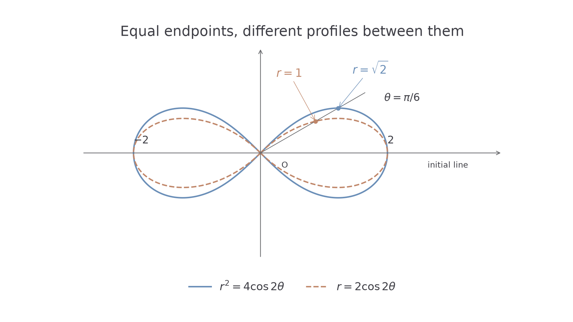
Equal tip radii and pole directions do not determine the whole curve

Worked example 13: sketching a lemniscate

Question. Give the key sketch features of $r^2=4\cos2\theta$ , with $r\ge0$ .

Plan. Find where a real radius exists, then take the positive square root at key angles.

\begin{aligned} r&=2\sqrt{\cos2\theta} && \text{non-negative root} \\ r(0)&=r(\pi)=2 && \text{horizontal tips} \\ r(\pi/4)&=0 && \text{right-loop endpoint} \\ r(\pi/6)&=2\sqrt{1/2}=\sqrt2 && \text{intermediate ray} \end{aligned}

Why this step? Taking the square root is essential. Using $r=2\cos2\theta$ would give the inner dashed curve in the diagram.

Answer. Two horizontal loops, symmetric about both axes, using $[-\pi/4,\pi/4]$ and $[3\pi/4,5\pi/4]$ , with tips $(\pm2,0)$ .

Check. At $\theta=\frac\pi6$ , the Cartesian point is $(\frac{\sqrt6}{2},\frac{\sqrt2}{2})$ ; its squared distance is $2$ , agreeing with $4\cos\frac\pi3$ .

Change only $a$ , from $2$ to $4$ ; the coefficient on the right changes from $4$ to $16$ .

Worked example 14: scaling a squared-radius curve

Question. Describe $r^2=16\cos2\theta$ , with $r\ge0$ .

Plan. Take the non-negative root and retain the same admissible angles.

\begin{aligned} r&=4\sqrt{\cos2\theta} && \text{square root of }16 \\ r(0)&=r(\pi)=4 && \text{tip radii} \\ r(\pi/6)&=4\sqrt{1/2}=2\sqrt2 && \text{intermediate radius} \end{aligned}

Why this step? Quadrupling the coefficient of $r^2$ doubles every radius. It does not quadruple the curve's linear size.

Answer. The preceding lemniscate enlarged by factor $2$ , with tips $(\pm4,0)$ , the same two admissible intervals and the same pole directions.

Check. The new intermediate radius $2\sqrt2$ has square $8=16\cos\frac\pi3$ .

The opening distinction now has a clear answer: $r=2\sec\theta$ is the vertical line $x=2$ , while $r=2$ is a circle centred at the pole. Decide what the radius does along its rays before naming a shape.

Watch out

Wrong: $r^2=16\cos2\theta$ implies $r=4\cos2\theta$ . Right: $r=4\sqrt{\cos2\theta}$ , with $\cos2\theta\ge0$ . The square root changes the whole profile between the key points.

A final comparison separates two shapes whose tips and pole directions agree.

Quick Recap

Use admissible angles, symmetry, pole directions and key radii together; label the pole and initial line.
Secant equations can give straight lines; constant radius gives a circle, while $r=2a\cos\theta$ gives a circle through the pole.
In $r=k\theta$ , each full turn adds $2\pi k$ to the radius.
Cardioids reach the pole; $r=a(3+2\cos\theta)$ has a positive minimum radius and an inward dimple.
Under $r\ge0$ , both double-angle families here have two horizontal loops, but the square root in the lemniscate changes its profile.

The opening secant equation gives a straight line; the constant-radius equation gives a circle.

Last Accessed

Core Pure Mathematics

Further Pure Mathematics 1

Further Pure Mathematics 2

Further Statistics 1

Further Statistics 2

Further Mechanics 1

Further Mechanics 2

Decision Mathematics 1

Decision Mathematics 2

CP 7.2 - Sketching polar curves

A secant equation can represent a line

Constant-radius circles and circles through the pole

A radius growing with angle gives a spiral

Cardioids have a cusp at the pole

A dimpled curve that misses the pole

Double-angle cosine with non-negative radius

A squared-radius equation gives a lemniscate

Quick Recap

Learn faster with Nova