D2 6.1, 6.2 - Recurrence models and first-order solutions | Edexcel A-Level Further Mathematics

A recurrence describes how a system changes one step at a time. You will build models with clear timing, solve first-order linear relations using complementary and particular solutions, apply conditions and recover a recurrence from a closed formula.

Define what one step means

A club retains $80\%$ of its members each month, then $30$ new members join. Must its membership grow without limit because people keep joining?

Not necessarily. Departures can balance arrivals. First pin down the timing: the same percentages and arrivals give a different model if the new members are also exposed to that month's departures.

You already know

Core Pure algebra lets you substitute a proposed formula into an equation and solve equations for unknown constants. A power such as $a^{n+1}$ equals $a\,a^n$ ; keeping the index visible will make these substitutions manageable.

A recurrence gives a term from earlier terms; an explicit or closed formula gives the term directly from its index. An initial condition tells you where the sequence starts.

Order and linearity

The order is the gap between the highest and lowest term indices after collecting terms. A first-order linear relation has the form $u_{n+1}-a u_n=f(n)$ , where the sequence terms appear to the first power and are not multiplied together.

It is homogeneous when $f(n)=0$ , and non-homogeneous when there is a non-zero term depending on $n$ alone. For example, $u_{n+1}=2u_n+3$ is linear; $u_{n+1}=u_n^2+3$ is not.

Use the same measurement instant for every $u_n$ . The subscript $0$ is often the starting value; it is not automatically the first completed period.

Worked example 1: departures before arrivals

Question. The club starts with $100$ members. Each month $80\%$ of the current members remain, then $30$ new members join. Define a recurrence and calculate the first two updated model values.

Plan. Let $u_n$ be membership after $n$ completed monthly updates, and translate the events in their stated order.

\begin{aligned} u_0&=100\\ u_{n+1}&=0.8u_n+30,\qquad n\ge0 &&\text{retain, then add}\\ u_1&=0.8(100)+30=110\\ u_2&=0.8(110)+30=118 \end{aligned}

Why this step? The $30$ arrivals enter after the retention calculation, so they are not multiplied by $0.8$ in this update.

Answer. The recurrence is $u_{n+1}=0.8u_n+30,\ u_0=100$ ; the next values are $110,118$ .

Check. The definition makes $u_1$ the result after one update, rather than the starting membership.

Worked example 2 changes only the order of events: arrivals now occur before retention.

Worked example 2: arrivals before departures

Question. Use the same starting membership and numbers, but let all $30$ arrivals join before the month's $80\%$ retention calculation.

Plan. Add the arrivals inside the retention bracket.

\begin{aligned} u_{n+1}&=0.8(u_n+30)=0.8u_n+24\\ u_1&=0.8(100+30)=104\\ u_2&=0.8(104+30)=107.2 \end{aligned}

Why this step? Both old and newly arrived members undergo retention in this revised model.

Answer. The new recurrence is $u_{n+1}=0.8u_n+24,\ u_0=100$ , giving $104,107.2$ .

Check. The smaller effective inflow $24$ explains why the updated membership is lower.

A fractional membership is a modelled aggregate or expected value, not a fraction of a literal person. State such limitations and avoid rounding every intermediate update unless the model explicitly requires it.

Watch out

Wrong: put $0.8(u_n+30)$ into a model whose arrivals occur after retention. Right: define the timing, then preserve the stated event order.

Change only the arrivals in Worked example 2.

Separate the lasting level from the initial effect

For $u_{n+1}=a u_n+b$ , try a constant particular solution $u_n=K$ . It must satisfy $K=aK+b$ . Subtracting that constant leaves a homogeneous relation for the remaining part.

Complementary function and particular solution

The complementary function solves the associated homogeneous recurrence, obtained by replacing its forcing term by zero. A particular solution is one formula satisfying the non-homogeneous recurrence.

Adding them gives the general solution. Applying the stated conditions selects one member of that family. Pearson also uses “particular solution” for the final sequence selected by those conditions; the working makes the meaning clear.

For the homogeneous equation $u_{n+1}-a u_n=0$ , trial $u_n=r^n$ gives $r-a=0$ , its auxiliary equation.

First-order constant-coefficient solution

For $u_{n+1}=a u_n+b$ , with constant $a\ne0,1$ ,

K=\frac{b}{1-a}, \qquad u_n=Aa^n+K

If $u_0=c$ , then $A=c-K$ . If $a=1$ , use $u_n=c+bn$ ; if $a=0$ , the recurrence directly gives $u_n=b$ for $n\ge1$ , with the separately stated $u_0$ . Not in the formula booklet: learn it.

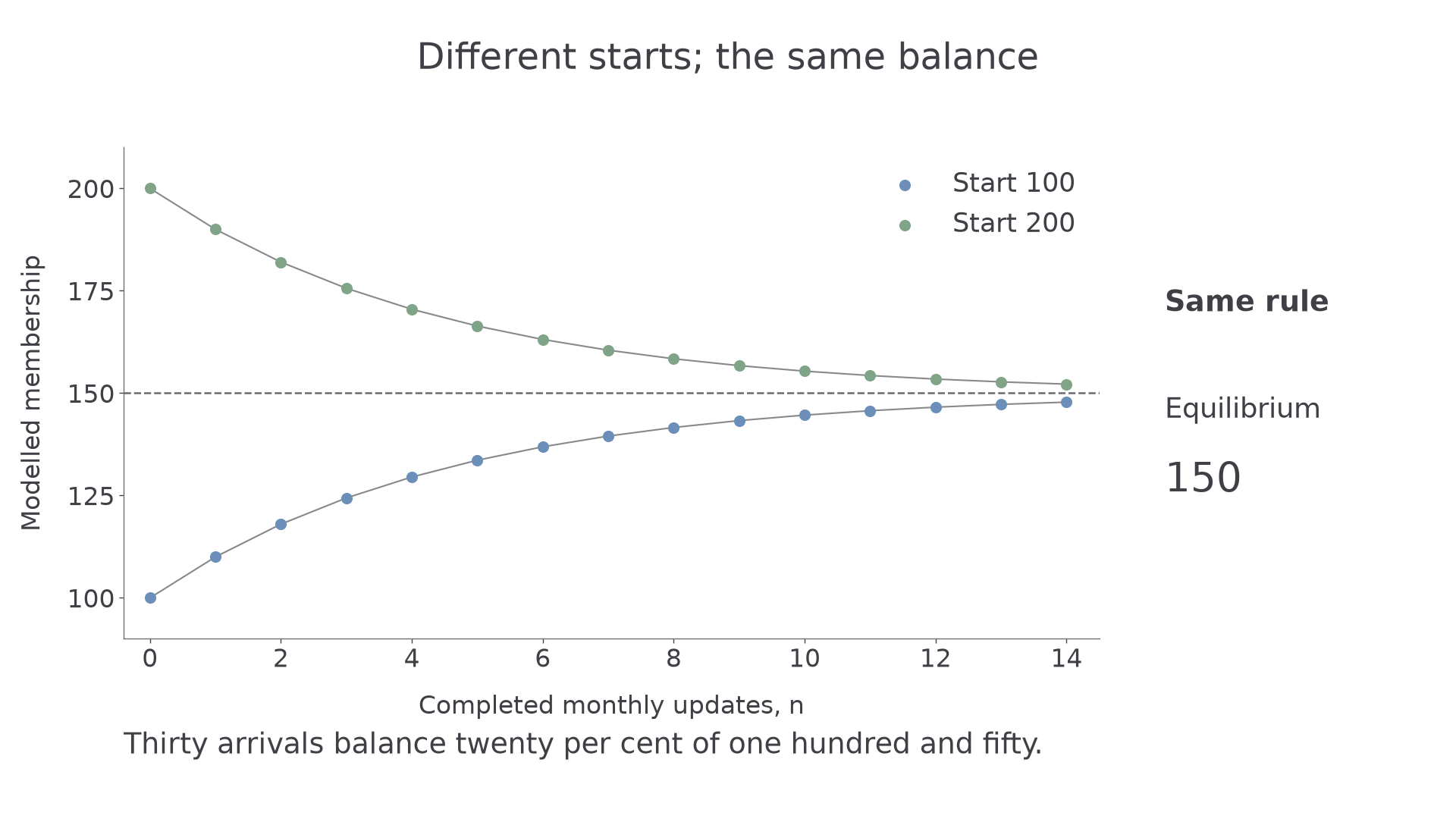
The constant $K$ is an equilibrium: starting there leaves every subsequent value there. Do not assume every equilibrium is approached; that depends on the multiplier $a$ .

Worked example 3: a constant inflow with a finite limit

Question. Solve the original club model $u_{n+1}=0.8u_n+30,\ u_0=100$ .

Plan. Find a constant particular solution, add the complementary function and fit the starting value.

\begin{aligned} K&=0.8K+30\implies K=150\\ r-0.8&=0\implies\text{C.F. }A(0.8)^n\\ u_n&=A(0.8)^n+150\\ 100&=A+150\implies A=-50\\ u_n&=150-50(0.8)^n \end{aligned}

Why this step? After subtracting $150$ , each remaining deviation is multiplied by $0.8$ at every update.

Answer. $u_n=150-50(0.8)^n$ ; the model approaches $150$ , so continued arrivals do not imply unlimited growth.

Check. $u_0=100$ and $u_1=150-40=110$ , matching direct iteration.

Worked example 4 changes only the starting membership from $100$ to $200$ .

Worked example 4: approaching the same level from above

Question. Solve the same recurrence with $u_0=200$ .

Plan. Keep the equilibrium and complementary function, changing only its coefficient.

\begin{aligned} u_n&=A(0.8)^n+150\\ 200&=A+150\implies A=50\\ u_n&=150+50(0.8)^n \end{aligned}

Why this step? The update rule fixes the equilibrium; the initial condition fixes the initial deviation.

Answer. $u_n=150+50(0.8)^n$ , approaching $150$ from above.

Check. Directly, $u_1=0.8(200)+30=190$ , agreeing with the formula.

When $|a|<1$ , $a^n$ tends to zero and the initial deviation disappears. A negative $a$ alternates its sign. When $|a|>1$ , a non-zero initial deviation grows in magnitude, so an equilibrium formula alone is not a stability claim. These are consequences of the power $a^n$ , not additional booklet formulas.

[DIAGRAM: asset_name: Different starts approach the same recurrence equilibrium; asset_slug: 9fm0-d2-192-equilibrium; caption: Retention and arrivals balance at one hundred and fifty; description: Exact discrete values for u next equals 0.8u plus thirty are plotted for starting values one hundred and two hundred. The lower sequence uses blue points and the upper sequence sage points, with thin joining guides. A grey horizontal line marks the equilibrium one hundred and fifty. The x axis counts completed monthly updates from zero. Labels state the two initial values and the common limiting level without crossing the curves]
Retention and arrivals balance at one hundred and fifty

Watch out

Wrong: use $30/(1+0.8)$ , or forget that $u_0=A+K$ . Right: solve $K=aK+b$ , then apply the initial condition to the whole general solution.

Change only the initial value again.

Match a polynomial forcing term

A polynomial forcing term suggests a polynomial particular solution of the same degree, with all lower-degree terms included. Substitute the whole trial at both $n+1$ and $n$ , then compare coefficients.

Polynomial trial rule

For $u_{n+1}-a u_n=P(n)$ , with constant $a\ne1$ , use a polynomial particular solution of the same degree as $P$ . For linear forcing try $pn+q$ ; for quadratic forcing try $pn^2+qn+r$ .

If $a=1$ , multiply this trial by $n$ , because constants already belong to the complementary function. Determine every trial coefficient by substitution. Not in the formula booklet: learn it.

Continue this lesson.

You’re previewing NovaLearn without an account. Create a free account to read the rest.

Create free account

Last Accessed

Core Pure Mathematics

Further Pure Mathematics 1

Further Pure Mathematics 2

Further Statistics 1

Further Statistics 2

Further Mechanics 1

Further Mechanics 2

Decision Mathematics 1

Decision Mathematics 2

D2 6.1, 6.2 - Recurrence models and first-order solutions

Define what one step means

Separate the lasting level from the initial effect

Match a polynomial forcing term

Continue this lesson.

Learn faster with Nova