FS1 6.1 - Contingency table tests | Edexcel A-Level Further Mathematics

Two categorical variables can be associated even when neither is numerical. You will calculate expected frequencies under independence, carry out a chi-squared contingency table test, combine sparse categories appropriately and explain why real counts cannot be replaced by percentages.

Expected counts when the variables are independent

Two samples have exactly the same percentages in every category. Must their chi-squared tests reach the same conclusion?

Keep that question open while building the test. Percentages describe the pattern; the number of independent observations also affects how much evidence the pattern provides.

You already know

A chi-squared test compares observed and expected counts using $T=\sum(O-E)^2/E$ . Large discrepancies give large $T$ ; expected cells below $5$ need attention. An upper-tail p-value or critical value determines significance, and a non-significant result does not prove the null hypothesis.

A contingency table classifies the same individuals in two ways. For example, each traveller has a day type and a travel choice. Each individual must occupy exactly one cell; repeated entries from one person are not fresh independent cases.

Contingency table and independence

A contingency table records frequencies for combinations of categories of two variables. Row and column totals are its marginal totals.

Under independence, the population proportion in a column is the same within every row. Thus the expected count for a row follows the overall column proportions.

Write $H_0$ : there is no association between the two named variables; $H_1$ : there is an association. “The variables are independent” is an equivalent null statement. Use association, rather than correlation, for these categorical variables.

Expected frequencies under independence

If row $i$ has total $R_i$ , column $j$ has total $C_j$ , and the grand total is $N$ ,

E_{ij}=\frac{R_iC_j}{N}

The expected table has the same row and column totals as the observed table. This calculation assumes the null hypothesis of independence. Not in the formula booklet: learn it.

For a fixed row, $C_j/N$ is the overall fraction in column $j$ ; multiplying by $R_i$ distributes that row according to the null pattern.

Worked example 1: equal row totals

Question. A random sample of independent travellers is classified by day type and choice of travel. Calculate the expected frequencies under no association.

Day type	Walk	Cycle	Bus	Total
Weekday	$18$	$12$	$30$	$60$
Weekend	$12$	$28$	$20$	$60$
Total	$30$	$40$	$50$	$120$

Plan. Multiply each row total by each column proportion.

\begin{aligned} E_{\text{weekday,walk}}&=\frac{60(30)}{120}=15\\ E_{\text{weekday,cycle}}&=\frac{60(40)}{120}=20\\ E_{\text{weekday,bus}}&=\frac{60(50)}{120}=25 \end{aligned}

Both row totals are $60$ , so the expected table is:

Day type	Walk	Cycle	Bus	Total
Weekday	$15$	$20$	$25$	$60$
Weekend	$15$	$20$	$25$	$60$
Total	$30$	$40$	$50$	$120$

Why this step? Independence makes the proportions equal across rows; it does not require equal expectations across different columns.

Answer. The two expected rows are both $15,20,25$ .

Check. All original margins are preserved and the minimum expectation is $15$ , safely above $5$ .

Worked example 2 changes only the balance between the row totals, retaining column totals $30,40,50$ and grand total $120$ .

Worked example 2: unequal row totals

Question. A sample instead has row totals $40$ weekday and $80$ weekend travellers. The column totals are unchanged. Calculate the expected table.

Plan. Use the new row totals with the same overall column proportions.

\begin{aligned} (E_{\text{weekday,walk}},E_{\text{weekday,cycle}},E_{\text{weekday,bus}}) &=40\left(\frac{30}{120},\frac{40}{120},\frac{50}{120}\right)\\ &=\left(10,\frac{40}{3},\frac{50}{3}\right)\\ (E_{\text{weekend,walk}},E_{\text{weekend,cycle}},E_{\text{weekend,bus}}) &=80\left(\frac{30}{120},\frac{40}{120},\frac{50}{120}\right)\\ &=\left(20,\frac{80}{3},\frac{100}{3}\right) \end{aligned}

Why this step? The larger row needs twice the expected counts, while the expected proportions stay the same.

Answer. The expected rows are $(10,40/3,50/3)$ and $(20,80/3,100/3)$ .

Check. The first row sums to $40$ , the second to $80$ , and corresponding cells sum to $30,40,50$ . Fractions need not be rounded to whole people.

The diagram contrasts actual counts with the independence model for the first table.

[DIAGRAM: asset_name: Observed and independent expected counts; asset_slug: 9fm0-fs1-112-independence; caption: Under independence each row follows the overall column proportions; description: Two clearly separated two-by-three frequency tables have weekday and weekend rows and walk, cycle and bus columns. The observed table contains rows 18,12,30 and 12,28,20; the expected table contains two rows 15,20,25. Both display row totals 60 and column totals 30,40,50 with grand total 120. A footer shows the example calculation 60 times 40 divided by 120 equals 20, and states that expected margins are unchanged]
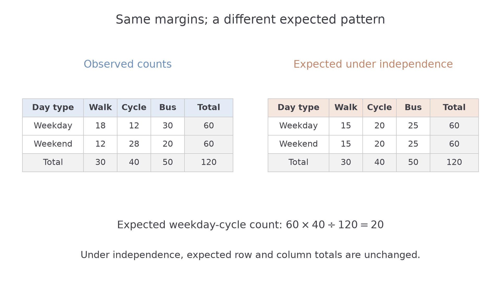
Under independence each row follows the overall column proportions

To check whether every expected count is large enough, the smallest row total and smallest column total give the smallest product $R_iC_j/N$ . The smallest observed entry need not be in that cell.

Watch out

Wrong: divide the total equally among all cells, choose the smallest observed cell to check validity, or round an expected count to an integer. Right: use the margins and retain precision.

Change the row balance again.

Testing for an association

Once the expected table is ready, calculate the same discrepancy statistic as in goodness of fit, including every interior cell. Row totals, column totals and the grand total are checks, not additional cells in the sum.

The degrees of freedom reflect the margins. In a $2$ by $2$ table with all margins fixed, choosing one cell determines the other three. More generally, only the top-left block of $(r-1)(c-1)$ cells can be chosen freely.

Contingency table degrees of freedom

For a retained table with $r$ rows and $c$ columns, using the usual independence test,

\nu=(r-1)(c-1)

Use $T$ approximately distributed as $\chi^2_\nu$ , with adequate expected frequencies and independent observations. The marginal-proportion fitting is already allowed for by this formula; do not subtract it again. Not in the formula booklet: learn it.

Use the upper chi-squared tail, just as before. A significant result supports an association between the named population variables; it does not identify a causal direction.

Worked example 3: evidence of an association

Question. Test for an association between day type and travel choice in Worked example 1, using a $5\%$ significance level.

Plan. State contextual hypotheses, calculate the six contributions and use $\nu=2$ .

\begin{aligned} H_0&:\ \text{day type and travel choice are independent}\\ H_1&:\ \text{day type and travel choice are associated}\\ T&=\frac{(18-15)^2}{15}+\frac{(12-20)^2}{20} +\frac{(30-25)^2}{25}\\ &\quad+\frac{(12-15)^2}{15}+\frac{(28-20)^2}{20} +\frac{(20-25)^2}{25}\\ &=0.6+3.2+1+0.6+3.2+1=9.6\\ \nu&=(2-1)(3-1)=2,\qquad c=5.991 \end{aligned}

Why this step? Six cells do not give $6-1$ degrees of freedom: the row and column margins impose more restrictions.

Answer. Since $9.6>5.991$ , reject $H_0$ . There is sufficient evidence at the $5\%$ level of an association between day type and travel choice.

Check. All expectations are at least $15$ . The upper-tail p-value is $0.0082297\ldots<0.05$ , giving the same decision.

Worked example 4 changes only the observed interior counts, preserving all margins and hence the expected table.

Worked example 4: a smaller discrepancy with the same margins

Question. Repeat the test with observed rows $16,18,26$ and $14,22,24$ , retaining the same day-type and travel-choice categories.

Plan. Keep expected rows $15,20,25$ and recalculate $T$ .

\begin{aligned} T&=\frac{1^2}{15}+\frac{(-2)^2}{20}+\frac{1^2}{25} +\frac{(-1)^2}{15}+\frac{2^2}{20}+\frac{(-1)^2}{25}\\ &=0.613333\ldots\\ \nu&=2,\qquad 0.613333\ldots<5.991 \end{aligned}

Why this step? The margins determine the null expectations, but the interior pattern determines how far the observations depart from them.

Answer. Do not reject $H_0$ . There is insufficient evidence of an association between day type and travel choice at $5\%$ .

Check. The calculator upper-tail p-value is $0.7358958\ldots>0.05$ . This does not establish that the variables are independent.

A calculator can evaluate $T$ or its p-value, but the expected table, degrees of freedom and contextual conclusion must still be clear.

Watch out

Wrong: use $\nu=6-1=5$ because the table has six interior cells. The fixed row and column margins impose additional restrictions. Right: use $\nu=(2-1)(3-1)=2$ , and sum the statistic over the interior cells only, excluding the totals.

The numerical comparison still needs a statement about the two population variables.

Exam tip

Keep both variables in the hypotheses and conclusion. “Reject” alone is incomplete; “there is a correlation” is inappropriate for an ordinary test of these categorical variables.

Move the cells a little further from independence.

Continue this lesson.

You’re previewing NovaLearn without an account. Create a free account to read the rest.

Create free account

Last Accessed

Core Pure Mathematics

Further Pure Mathematics 1

Further Pure Mathematics 2

Further Statistics 1

Further Statistics 2

Further Mechanics 1

Further Mechanics 2

Decision Mathematics 1

Decision Mathematics 2

FS1 6.1 - Contingency table tests

Expected counts when the variables are independent

Testing for an association

Continue this lesson.

Learn faster with Nova