FS1 5.1 - Sample means from other distributions | Edexcel A-Level Further Mathematics

Individual counts and waiting times can be far from normally distributed, yet their averages can have a useful normal approximation. You will apply the Central Limit Theorem, distinguish variance from standard error, and decide whether a sample and its context support the approximation.

Averaging changes the distribution and its spread

A first-success wait with success probability $1/4$ is most likely to last just one trial. Can the average of many such waits behave like a bell-shaped variable centred at four trials?

Yes, provided the waits are independent and follow the same model. Averages vary less than individual observations, and their shape can become much closer to normal even though the original waiting-time distribution stays skewed.

You already know

From A-level Mathematics, $\mathrm N(\mu,\sigma^2)$ names a normal distribution using its mean and variance; normal probabilities and inverse normal calculations use standard deviation. From earlier FS1 lessons, a geometric trial count has mean $1/p$ and variance $(1-p)/p^2$ , and different distributions can share a mean while having different variances.

Imagine repeating the whole sampling experiment, taking a fresh batch each time. The batch mean changes from sample to sample. Its distribution is the object we are about to approximate.

Sample mean and standard error

For independent observations $X_1,\ldots,X_n$ from the same population,

\overline X=\frac{X_1+\cdots+X_n}{n}

is the sample mean. Upper-case $\overline X$ is a random variable before the sample is observed; lower-case $\overline x$ is its realised value.

The standard error of the mean is the standard deviation of $\overline X$ , measuring variation between repeated sample means.

Two exact moment results explain why averages settle down. A further result describes their approximate shape.

Mean and variance of an independent sample mean

For a random sample of size $n$ from a population with finite mean $\mu$ and finite variance $\sigma^2$ ,

\mathrm E(\overline X)=\mu,\qquad \operatorname{Var}(\overline X)=\frac{\sigma^2}{n}

The observations must be independent and have the same population moments. These equalities are exact; they do not require a normal population or a large sample. In the formula booklet.

Taking the square root gives standard error $\sigma/\sqrt n$ . This consequence of the printed variance formula is not separately named in the booklet; the same denominator appears in its normal-population standardisation formula.

Central Limit Theorem for a sample mean

For independent observations from the same population with finite mean $\mu$ and finite variance $\sigma^2>0$ , when $n$ is sufficiently large,

\overline X\ \text{is approximately}\ \mathrm N\!\left(\mu,\frac{\sigma^2}{n}\right),\qquad Z=\frac{\overline X-\mu}{\sigma/\sqrt n} \ \text{is approximately}\ \mathrm N(0,1)

This extends the normal approximation to sample means from other distributions. No proof is required. Not in the formula booklet: learn it.

The booklet's exact standardisation formula assumes a normal population. If the original population is normal, $\overline X$ is exactly normal for every sample size. For another population, the Central Limit Theorem supplies an approximation for large $n$ . If $\sigma^2=0$ , every observation and every mean is constant; do not divide by zero to form $Z$ .

Worked example 1: the distribution of an average wait

Question. Independent first-success trial counts $X_i$ each follow $\operatorname{Geo}(1/4)$ . For a sample of $100$ counts, state an approximate distribution for $\overline X$ and find its standard error.

Plan. Find the population moments, divide the variance by the sample size, and apply the Central Limit Theorem.

\begin{aligned} \mu&=\frac1{1/4}=4,\qquad \sigma^2=\frac{3/4}{(1/4)^2}=12 &&\text{population moments}\\ \operatorname{Var}(\overline X)&=\frac{12}{100}=0.12 &&\text{variance of the mean}\\ \overline X&\ \text{is approximately}\ \mathrm N(4,0.12) &&\text{independent sample; large }n\\ \operatorname{se}(\overline X)&=\sqrt{0.12}=0.346410\ldots &&\text{square root of the variance} \end{aligned}

Why this step? The random variable is an average of $100$ waits, so the normal model needs variance $12/100$ , rather than the individual variance $12$ .

Answer. Approximately $\mathrm N(4,0.12)$ , with standard error $0.346$ trials to three significant figures.

Check. The centre is still $4$ , and the standard error is one tenth of the individual standard deviation $\sqrt{12}$ .

Worked example 2 changes only the sample size, from $100$ to $400$ . Four times as many observations will halve the standard error.

Worked example 2: four times the sample size

Question. For the same geometric population, state an approximate distribution of the mean of $400$ independent waits and its standard error.

Plan. Keep the population moments and replace $n$ .

\begin{aligned} \operatorname{Var}(\overline X)&=\frac{12}{400}=0.03 &&\text{new sample size}\\ \overline X&\ \text{is approximately}\ \mathrm N(4,0.03) &&\text{same centre, smaller spread}\\ \operatorname{se}(\overline X)&=\sqrt{0.03}=0.173205\ldots &&\text{new standard error} \end{aligned}

Why this step? Variance decreases in proportion to $1/n$ , while standard error decreases in proportion to $1/\sqrt n$ .

Answer. Approximately $\mathrm N(4,0.03)$ , with standard error $0.173$ trials.

Check. $0.03=0.12/4$ , and $\sqrt{0.03}=\sqrt{0.12}/2$ . The population's own variance remains $12$ .

This square-root effect is a useful surprise: halving the standard error requires four times as much data, not twice as much. It follows exactly from the sample-mean variance, rather than depending on the normal approximation.

[DIAGRAM: asset_name: Skewed waits and approximately normal averages; asset_slug: 9fm0-fs1-110-averaging; caption: Individual waits stay skewed while sample means concentrate around the same population mean; description: The left panel shows exact geometric probabilities for success probability one quarter on trials one to fifteen, with the decreasing first bar highlighted and mean four marked. The right panel shows the Central Limit Theorem normal density models for sample means of twenty-five and one hundred independent waits, both centred at four. The curve for one hundred has half the standard error and is narrower. The panels explicitly use probability and density scales respectively, and a note states that the right curves are approximations]
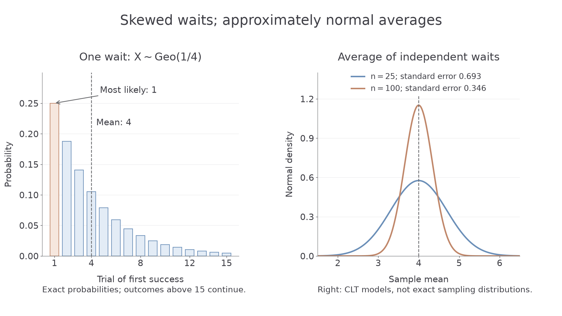
Individual waits stay skewed while sample means concentrate around the same population mean

The right-hand curves model variation between fresh sample means. They do not claim that the trial count for one experiment has become normal.

Watch out

Wrong: $\overline X$ has variance $\sigma/\sqrt n$ , or standard deviation $\sigma/n$ . Right: put $\sigma^2/n$ in $\mathrm N(\mu,\sigma^2/n)$ , and use its square root $\sigma/\sqrt n$ in a normal calculation.

Reduce the sample size while retaining the same population.

Probabilities for averages of waiting times

Start with the distribution of one observation, obtain its moments, then move to the distribution of the average. This order prevents the success probability, target number of successes and sample size from being confused.

For a sample of geometric waits, $p$ determines each wait's moments. For negative binomial waits, both $r$ and $p$ do. The sample size $n$ is how many complete waiting experiments are averaged.

Worked example 3: an unusually high average first-success wait

Question. Independent trials succeed with probability $1/4$ . Each of $100$ independent experiments ends at its first success. Use the Central Limit Theorem to estimate the probability that the mean trial count exceeds $4.6$ , to four decimal places.

Plan. Use the sample-mean model from Worked example 1 and standardise the upper tail.

\begin{aligned} \overline X&\ \text{is approximately}\ \mathrm N(4,0.12) &&\text{geometric moments; }n=100\\ \mathrm P(\overline X>4.6) &\approx\mathrm P\!\left(Z>\frac{4.6-4}{\sqrt{0.12}}\right) &&\text{divide by standard error}\\ &=\mathrm P(Z>1.732050\ldots) &&\text{retain full precision}\\ &=0.0416322\ldots &&\text{normal upper tail} \end{aligned}

Why this step? A normal calculator requires standard deviation $\sqrt{0.12}$ , not variance $0.12$ .

Answer. The estimated probability is $0.0416$ .

Check. The threshold is above the population mean, so the upper-tail probability is below $0.5$ ; it lies about $1.73$ standard errors above the centre.

Worked example 4 changes only the success target of each experiment, from the first success to the third. The success probability, sample size and excess of the threshold over its own mean remain the same.

Worked example 4: averaging third-success waits

Question. Each of $100$ independent experiments now continues until the third success, with success probability $1/4$ on every independent trial. Estimate the probability that the mean trial count exceeds $12.6$ , to four decimal places.

Plan. Use the negative binomial moments of one experiment, then divide its variance by $100$ .

\begin{aligned} X_i&\sim\operatorname{NB}(3,1/4) &&\text{third-success trial count}\\ \mu&=\frac3{1/4}=12,\qquad \sigma^2=\frac{3(3/4)}{(1/4)^2}=36 &&\text{individual moments}\\ \overline X&\ \text{is approximately}\ \mathrm N(12,0.36) &&36/100=0.36\\ \mathrm P(\overline X>12.6) &\approx\mathrm P\!\left(Z>\frac{12.6-12}{0.6}\right) &&\sqrt{0.36}=0.6\\ &=\mathrm P(Z>1)=0.1586552\ldots &&\text{normal upper tail} \end{aligned}

Why this step? Increasing the success target changes both population moments. Reusing variance $12$ from the first-success model would make the average look too concentrated.

Answer. The estimated probability is $0.1587$ .

Check. The threshold is one standard error above the new mean. Its upper tail is therefore larger than the tail at about $1.73$ standard errors in Worked example 3.

Continue this lesson.

You’re previewing NovaLearn without an account. Create a free account to read the rest.

Create free account

Last Accessed

Core Pure Mathematics

Further Pure Mathematics 1

Further Pure Mathematics 2

Further Statistics 1

Further Statistics 2

Further Mechanics 1

Further Mechanics 2

Decision Mathematics 1

Decision Mathematics 2

FS1 5.1 - Sample means from other distributions

Averaging changes the distribution and its spread

Probabilities for averages of waiting times

Continue this lesson.

Learn faster with Nova