FS2 5.4, 5.5 - Testing the difference between two means | Edexcel A-Level Further Mathematics

Two sample means vary even when their population means have a stated difference. You will test that difference using independent normal samples with known variances, choose the correct tail, and extend the method to large samples with estimated variances.

Build the sampling model for the difference

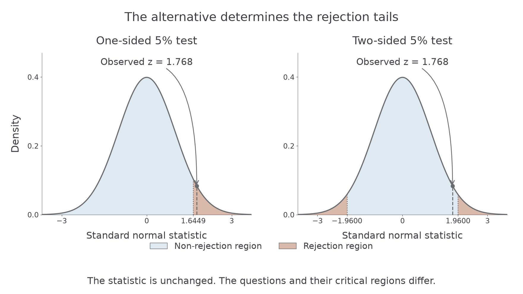
Can the same data be significant in a one-sided $5\%$ test but not in a two-sided $5\%$ test? Yes. A standardised difference of about $1.768$ exceeds the one-sided critical value $1.6449$ , but not the two-sided value $1.9600$ . The tests ask different questions.

That is not a licence to choose an alternative after looking at the result. State the question first; it determines which outcomes count as evidence.

You already know

Independent normal means remain normal when subtracted. Their mean difference is the difference of their population means, while their variance contributions add. A sample variance $s^2$ estimates a population variance; it is not automatically a known population quantity.

Let $\mu_X-\mu_Y=\delta$ be the population mean difference. For independent samples of sizes $n_X,n_Y$ from normal populations,

\bar X-\bar Y\sim\mathrm N\left( \delta,\frac{\sigma_X^2}{n_X}+\frac{\sigma_Y^2}{n_Y} \right)

This follows from the preceding normal-combination result. The populations need not have equal variances.

Null and alternative hypotheses for a mean difference

The null hypothesis specifies a benchmark $H_0:\mu_X-\mu_Y=\delta_0$ . The alternative states the question: a greater difference, a smaller difference or a difference in either direction. Hypotheses concern population means, not the two observed sample means. The common benchmark is $0$ , but a non-zero stated difference is equally valid.

The standard error measures the sampling spread of the difference. Under the null, subtract its stated centre before standardising.

Known-variance difference statistic

For independent normal samples with known population variances, under $H_0:\mu_X-\mu_Y=\delta_0$ ,

Z= \frac{(\bar X-\bar Y)-\delta_0} {\sqrt{\sigma_X^2/n_X+\sigma_Y^2/n_Y}} \sim\mathrm N(0,1)

In the formula booklet.

At the $5\%$ level, the appropriate normal comparisons are:

Alternative	Rejection rule	p-value from observed $z$
$\mu_X-\mu_Y>\delta_0$	$z>1.6449$	$1-\Phi(z)$
$\mu_X-\mu_Y<\delta_0$	$z<-1.6449$	$\Phi(z)$
$\mu_X-\mu_Y\ne\delta_0$	$	z

Here $\Phi(z)=\mathrm P(Z\le z)$ . A p-value is the probability, under $H_0$ , of a result at least as extreme in the direction or directions specified by $H_1$ . Compare it with the significance level. These test rules are consequences of the supplied normal distribution and percentage points, rather than separately printed test recipes.

Key idea

Keep one convention throughout: define the difference as $X$ minus $Y$ , state the matching population hypothesis, then use its corresponding tail.

Translate the claim into population parameters before using any data.

Use the stated alternative with the known variances

A complete test states its hypotheses, sampling model, statistic, critical comparison and contextual conclusion. Show which population is being subtracted; a sign change without a matching tail change can reverse the conclusion.

For the next pair, component lengths in populations $X$ and $Y$ are normal. Independent random samples give

n_X=36,\quad \bar x=54.5\,\mathrm{mm},\quad \sigma_X=6\,\mathrm{mm}

n_Y=64,\quad \bar y=50\,\mathrm{mm},\quad \sigma_Y=8\,\mathrm{mm}

The two population standard deviations are known.

Worked example 1: a one-sided difference claim

Question. Test, at the $5\%$ level, whether $\mu_X$ exceeds $\mu_Y$ by more than $2\,\mathrm{mm}$ .

Plan. Use benchmark $2$ , calculate the standard error from the two known variances, and compare the signed statistic with the upper-tail critical value.

H_0:\mu_X-\mu_Y=2,\qquad H_1:\mu_X-\mu_Y>2

\begin{aligned} \operatorname{se}(\bar X-\bar Y) &=\sqrt{\frac{6^2}{36}+\frac{8^2}{64}} =\sqrt2 && \text{independent mean variances}\\ z&=\frac{(54.5-50)-2}{\sqrt2} =\frac{2.5}{\sqrt2}=1.767766\ldots && \text{subtract the null difference}\\ 1.767766\ldots&>1.6449 && \text{upper }5\%\text{ critical value} \end{aligned}

Why subtract $2$ ? The null sampling model is centred at a difference of $2$ , rather than at zero.

Answer. Reject $H_0$ . There is sufficient evidence at the $5\%$ level that population $X$ 's mean length exceeds population $Y$ 's by more than $2\,\mathrm{mm}$ .

Check. The upper-tail p-value is $0.0385499\ldots<0.05$ , agreeing with the critical-value decision.

Worked example 2 changes only the alternative, from a greater difference to a difference in either direction. The data, benchmark and level remain fixed.

Worked example 2: the same data with a two-sided question

Question. Test, at the $5\%$ level, whether the population mean difference differs from $2\,\mathrm{mm}$ .

Plan. Keep the statistic and use both tails, each with probability $0.025$ .

H_0:\mu_X-\mu_Y=2,\qquad H_1:\mu_X-\mu_Y\ne2

\begin{aligned} z&=\frac{(54.5-50)-2}{\sqrt2}=1.767766\ldots && \text{unchanged sampling calculation}\\ |z|&<1.9600 && \text{two-sided }5\%\text{ critical comparison}\\ p&=2\,\mathrm P(Z>1.767766\ldots) =0.0770998\ldots && \text{both equally extreme tails} \end{aligned}

Why does the decision change? The two-sided test reserves probability for evidence in either direction, making each individual tail smaller.

Answer. Do not reject $H_0$ . There is insufficient evidence at the $5\%$ level that the population mean difference differs from $2\,\mathrm{mm}$ .

Check. $p>0.05$ . The statistic lies between $1.6449$ and $1.9600$ , exactly the range where these two questions can give different decisions.

The opening puzzle is therefore consistent: the same observation is being judged against different pre-specified alternatives.

[DIAGRAM: asset_name: One-sided and two-sided normal rejection regions; asset_slug: 9fm0-fs2-130-test-tails; caption: The same observed statistic can cross a one-sided cutoff while remaining inside two-sided cutoffs; description: Two panels show the standard normal density with pale blue non-rejection regions and pale clay rejection tails. In the one-sided five percent panel, the right rejection tail begins at one point six four four nine. In the two-sided five percent panel, the rejection tails begin at minus and plus one point nine six zero zero. A grey observed-statistic guide at approximately one point seven six eight is in the right rejection region of the first panel and inside the central region of the second. Grey curve outlines, ink labels and full-opacity pointers keep the comparisons clear.]
The same observed statistic can cross a one-sided cutoff while remaining inside two-sided cutoffs

Watch out

Wrong: use $|z|$ and a positive critical value for every test, or choose a one-sided alternative after seeing a favourable sign. Right: choose the alternative first and preserve its direction throughout.

Change only the alternative's direction once more.

Continue this lesson.

You’re previewing NovaLearn without an account. Create a free account to read the rest.

Create free account

Last Accessed

Core Pure Mathematics

Further Pure Mathematics 1

Further Pure Mathematics 2

Further Statistics 1

Further Statistics 2

Further Mechanics 1

Further Mechanics 2

Decision Mathematics 1

Decision Mathematics 2

FS2 5.4, 5.5 - Testing the difference between two means

Build the sampling model for the difference

Use the stated alternative with the known variances

Continue this lesson.

Learn faster with Nova