FS2 1.1 - Least squares regression lines
A regression line is chosen by a precise measure of its errors, rather than by eye. You will explain least squares, calculate the regression of a response on an explanatory variable and recover a model when the data have been coded.
What makes a line the best fit?
Can the best-fitting straight line miss every data point?
Yes. For the three points , the least squares line is , and none of the points lies on it. “Best” refers to the combined prediction errors, not the number of points hit exactly.
You already know
From A-level Mathematics, a scatter diagram shows the relationship between two variables, and a regression line can estimate a response within a suitable model. Interpolation is generally more defensible than extrapolation; an association does not establish causation. Here we calculate the line's coefficients and explain the least squares criterion.
Choose the response before fitting. In regression of on , values of are used to estimate . The errors are measured in the -direction.
Fitted value, residual and least squares
For a proposed line , the fitted value at observation is . Its residual is
The least squares regression line of on minimises , the sum of squared vertical residuals, over choices of and .
A positive residual means the point is above the line; a negative one means it is below. Squaring prevents opposite signs from cancelling. Least squares does not minimise perpendicular distances to the line.
For the opening points, the fitted values are . The residuals are
Their squares sum to . In contrast, the line passes through two points but has residuals , with squared sum . Hitting more points does not necessarily give a smaller total squared error.
[DIAGRAM: asset_name: The best line need not pass through a point; asset_slug: 9fm0-fs2-118-vertical-residuals; caption: Least squares minimises squared vertical residuals, rather than the number of missed points; description: A scatter plot shows the three exact points zero comma one, one comma two and two comma two. The line y equals seven sixths plus x over two passes between them. Pale clay vertical segments join each observed point to its fitted value, with residual labels minus one sixth, plus one third and minus one sixth positioned clear of the points and line. The sum of squared residuals is stated as one sixth]
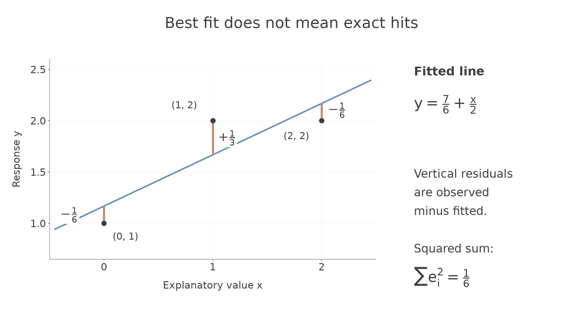
The formulas in the next part identify this minimum directly. No trial-and-error search through possible lines is needed.
Key idea
Least squares balances squared vertical prediction errors across the entire dataset; it need not pass through any individual observation.
Check the criterion itself.
Calculating the coefficients from summaries
The line depends on how the two variables vary together, measured relative to the variation in the explanatory variable.
First find the sample means and the centred sums. The expression means square the total; it is different from , the sum of individual squares.
Centred sums for regression
For paired observations,
Use the same paired observations in every sum. In the formula booklet.
The denominator for the slope is , because the response is being fitted on . Naming different variables does not change this response-versus-explanatory distinction.
Least squares line of y on x
If , the least squares line is
It therefore passes through the mean point . Pearson may write the fitted equation as . In the formula booklet.
When all -values are equal, , so these observations do not determine a unique slope. If while , the fitted slope is zero; that alone does not mean all observations lie on the line.
Worked example 1: a positive fitted slope
Question. Eight paired observations have
Find the regression line of on .
Plan. Calculate the means and centred sums, then the slope and intercept.
Why this step? The slope divides the centred cross-product by the explanatory sum of squares, not by the number of observations.
Answer. .
Check. Substituting the mean gives the mean response .
Continue this lesson.
You’re previewing NovaLearn without an account. Create a free account to read the rest.
Create free account