FS2 2.1, 2.2 - Density and cumulative distribution functions
A continuous model assigns probabilities to intervals by measuring area. You will use a probability density function to find probabilities, construct a cumulative distribution function with the correct branches, and move between the two functions by integration and differentiation.
Density is height; probability is area
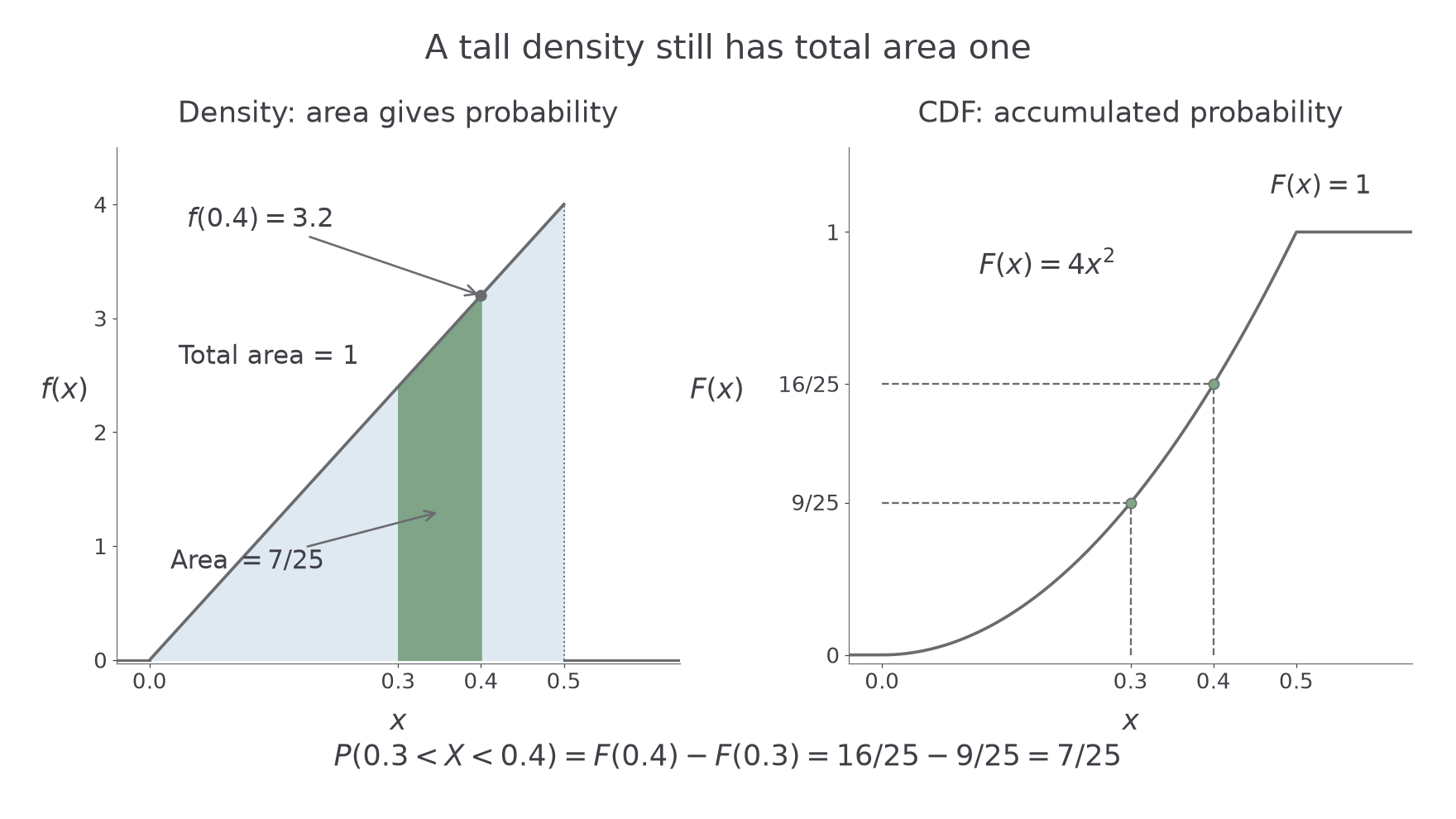
A probability model has density . Has something gone wrong because ? It sounds suspicious until you ask what the vertical axis measures.
Imagine a histogram whose bar areas are relative frequencies, so its total area is . A narrow class can have a tall bar without containing more than all the observations. A frequency polygon smooths the outline; a density curve takes the same area idea into a continuous model.
You already know
From A-level Mathematics, a definite integral measures area under a non-negative curve. If , then .
Here is the model behind the opening question:
Its whole triangular area is . Although its greatest height is , every interval probability is an area between and .
[DIAGRAM: asset_name: A tall density and its cumulative area; asset_slug: 9fm0-fs2-120-density-cdf; caption: Density height can exceed one while every accumulated probability stays between zero and one; description: Two labelled coordinate panels describe the density f of x equals eight x from zero to one half and zero elsewhere. The left panel shows its triangular area one and shades the interval from three tenths to four tenths in sage, with shaded area seven twenty-fifths. The right panel shows the CDF zero below zero, four x squared from zero to one half, and one thereafter. Dashed guides mark F of three tenths equals nine twenty-fifths and F of four tenths equals sixteen twenty-fifths, whose difference is seven twenty-fifths. All labels and arrows are full-opacity grey.]
Continuous random variable and probability density function
A continuous random variable is modelled by a density , with and total area . The probability of an interval is its area under the density. For example, a measured waiting time can be continuous; a count of waiting customers is discrete.
A curve with total area but a negative region is not a density. Both conditions matter.
Probabilities from a density
For a continuous random variable with density ,
Use the intersection of the requested interval with the support, the region where the density can be non-zero. These area and normalisation rules follow from the density model.
Not in the formula booklet: learn it.
A single point has no width, hence no area: . This does not mean a continuous observation cannot occur; it means probability is spread over intervals rather than assigned as positive masses to individual points. Consequently, changing an endpoint from strict to inclusive does not alter a continuous probability. Changing a density's value at one isolated point also leaves all its probabilities unchanged.
Key idea
The height is a density, not . If is measured in seconds, density has units of inverse seconds; integrating over seconds gives a dimensionless probability.
Keep that distinction in mind when reading the vertical axis.
Find a density constant and integrate over its support
An unknown density constant is fixed by total area . Write the support beside the integral before doing any calculus. An infinite endpoint means taking a limit, not substituting infinity as an ordinary number.
Worked example 1: an infinite right-hand tail
Question. A continuous random variable has density for , and otherwise. Find and .
Plan. Normalise over , then integrate the resulting density from to .
Why start at ? There is no probability below the support, so the requested event is exactly .
Answer. , and .
Check. The density is non-negative. The complementary tail has area , so the two areas add to .
Worked example 2 changes only the lower support endpoint. The old constant cannot survive unchanged.
Worked example 2: moving the start of the support
Question. Now for , and otherwise. Find and .
Plan. Repeat normalisation with lower limit , then use that same lower limit in the probability integral.
Why change the constant? Removing removes area; the remaining curve must become taller to keep total probability .
Answer. , and .
Check. Its tail above also has area . The event and its complement have equal areas.
The calculus is ordinary integration. The modelling work is choosing the correct limits and checking the curve's sign.
Watch out
Wrong: integrate from because probabilities start at zero. Right: integrate over the stated support. Here below , and the formula is not the density there.
Move the lower support endpoint once more.
Accumulate every earlier piece of area
A cumulative distribution function answers “how much probability has accumulated by this point?” Once a density changes formula, the area already collected does not disappear.
Cumulative distribution function
The cumulative distribution function, or CDF, is . It is non-decreasing, takes values between and , and has limits and at the two ends of the real line. For a continuous model it is continuous, even when the density has a jump.
The lower limit is the beginning of all accumulated probability, rather than a convenient integration constant.
Continue this lesson.
You’re previewing NovaLearn without an account. Create a free account to read the rest.
Create free account