FM2 4.2 - Simple harmonic motion of a particle | Edexcel A-Level Further Mathematics

Core Pure supplied the differential-equation solution for SHM. Here you will establish it from a force model, identify an unknown oscillation from measured motion, and choose times using the actual starting direction. You will also calculate durations within a cycle and connect the speed relation to kinetic and potential energy.

Prove SHM using displacement from equilibrium

Can a constant extra force move an oscillator's centre without changing its period? In an ideal linear restoring-force model, yes. The constant term shifts equilibrium; the coefficient of displacement controls the period. We will make that separation explicitly rather than trying to identify SHM from a sinusoidal-looking path.

You already know

Core Pure SHM has $\ddot x=-\omega^2x$ , with $\omega>0$ , and $x=A\cos\omega t+B\sin\omega t$ . Here x is signed displacement from equilibrium. Velocity is its derivative, and initial displacement and velocity fix separate constants. Variable-acceleration methods and Newton's law use the same signed axis.

To prove SHM, locate equilibrium first. If a question's position coordinate y is measured from another origin, solve the zero-resultant condition for its equilibrium value $y_0$ , then define $x=y-y_0$ . Since $y_0$ is constant, $\ddot x=\ddot y$ . The final equation must have a negative constant coefficient times x.

What establishes SHM

For displacement x from a fixed equilibrium,

\ddot x=-\omega^2x,\qquad \omega>0,\qquad T=\frac{2\pi}{\omega}

Acceleration is proportional to displacement and directed towards equilibrium. The coefficient of x is $-\omega^2$ , not $-\omega$ . A zero-amplitude solution is stationary equilibrium; a non-zero initial displacement or velocity produces the oscillation.

Not in the formula booklet: learn it.

The specification allows standard SHM formulae to be quoted without proof. They are not printed in the formula booklet, so you must know them. When asked to prove SHM in a situation, use the force equation to establish the restoring acceleration rather than merely quoting a sine or cosine solution.

[DIAGRAM: asset_name: A shifted equilibrium with unchanged restoring gradient; asset_slug: 9fm0-fm159-force-equilibrium; caption: A constant extra force shifts the zero-force point while leaving the restoring gradient unchanged; description: Two exact straight force-position graphs F equals12 minus3y and F equals18 minus3y have the same slope minus3 and cross the position axis at four and six metres. At points on either side of each equilibrium the force direction points back towards its own zero-force position.]
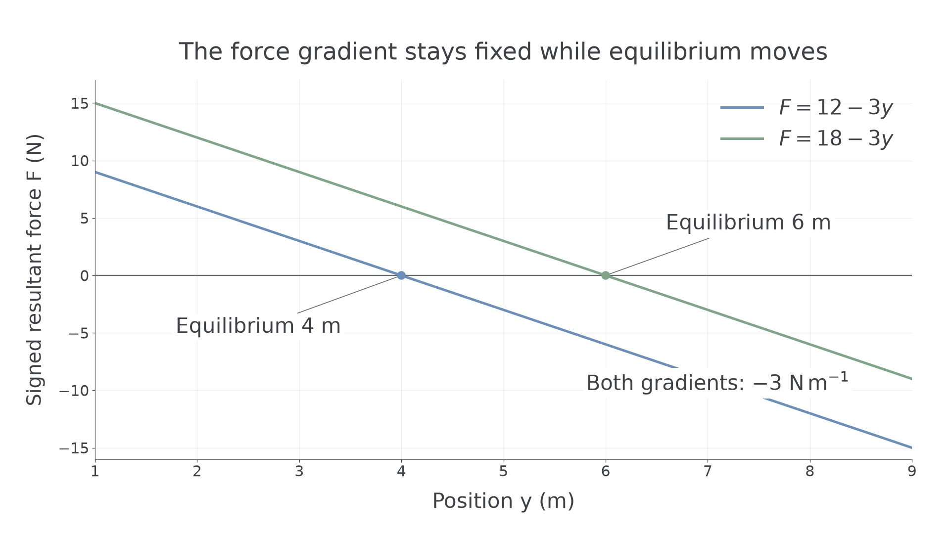
A constant extra force shifts the zero-force point while leaving the restoring gradient unchanged

Worked example 1: a shifted equilibrium

Question. A particle of mass $3\,\mathrm{kg}$ moves on a smooth straight guide. The resultant force in the positive y direction is $(12-3y)\,\mathrm{N}$ , where y is the numerical position in metres. Show that the motion about equilibrium is SHM and find its period.

Plan. Find the zero-force position, measure displacement from it, and apply Newton's law.

12-3y_0=0\Rightarrow y_0=4\,\mathrm{m}

Define $x=y-4$ . Then

3\ddot x=12-3(x+4)=-3x \Rightarrow\ddot x=-x

Why this step? The original acceleration $4-y$ is not proportional to y measured from the original origin. Translating to the equilibrium position removes the constant term.

Answer. The acceleration is towards equilibrium and proportional to x, with $\omega=1\,\mathrm{s^{-1}}$ . Thus the motion is SHM and $T=2\pi\,\mathrm{s}$ .

Check. For $x>0$ the force is negative; for $x<0$ it is positive. At $x=0$ the force vanishes, as equilibrium requires.

Change only the constant term of the force, from $12$ to $18\,\mathrm{N}$ .

Worked example 2: the centre moves but the restoring gradient stays fixed

Question. The same mass has resultant force $(18-3y)\,\mathrm{N}$ . Show that it executes SHM about its new equilibrium and find the period.

Plan. Recalculate the equilibrium, keeping the same mass and displacement coefficient.

18-3y_0=0\Rightarrow y_0=6\,\mathrm{m},\qquad x=y-6

3\ddot x=18-3(x+6)=-3x \Rightarrow\ddot x=-x

Why this step? The constant force changes the balance position but cancels when displacement is measured from that new balance position.

Answer. SHM about $y=6\,\mathrm{m}$ , still with $\omega=1\,\mathrm{s^{-1}}$ and $T=2\pi\,\mathrm{s}$ .

Check. The equilibrium has moved by $2\,\mathrm{m}$ , while the force gradient and mass are unchanged. This answers the opening question within the ideal linear model.

If the translated equation instead has a positive coefficient, such as $\ddot x=+x$ , the force points away from equilibrium. That is not SHM, even though the resultant is zero at one point.

Watch out

Wrong: claim that $\ddot y=4-y$ is SHM about $y=0$ , or identify $\omega$ directly from an unshifted force. Right: define displacement from the actual equilibrium, include the mass, and display $\ddot x=-\omega^2x$ .

Change only the constant force term again.

Use motion data to identify the oscillation

A greatest acceleration magnitude is positive. It is $a\omega^2$ for amplitude $a>0$ , rather than $-a\omega^2$ . A speed measurement at a known displacement gives another equation, allowing the two unknowns a and $\omega$ to be found together.

SHM motion relations

For amplitude $a>0$ , angular frequency $\omega>0$ and displacement x from equilibrium,

v^2=\omega^2(a^2-x^2),\qquad |v|_{\max}=a\omega,\qquad |\ddot x|_{\max}=a\omega^2

Also $T=2\pi/\omega$ , and physically $|x|\le a$ . These standard relations may be quoted; the squared-speed formula gives magnitude, not direction.

Not in the formula booklet: learn it.

Use exact values through the elimination. An algebraic negative amplitude root is inadmissible, and a proposed amplitude smaller than the measured displacement cannot describe that motion.

Worked example 3: acceleration and a speed measurement

Question. A particle has greatest acceleration magnitude $16\,\mathrm{m\,s^{-2}}$ . When it is $0.6\,\mathrm{m}$ from equilibrium its speed is $3.2\,\mathrm{m\,s^{-1}}$ . Find its amplitude and period.

Plan. Use the greatest acceleration to eliminate $\omega^2$ from the speed relation, then choose the positive amplitude.

a\omega^2=16,\qquad 3.2^2=\omega^2(a^2-0.6^2)

10.24a=16(a^2-0.36) \Rightarrow25a^2-16a-9=0 \Rightarrow(a-1)(25a+9)=0

The positive root is $a=1\,\mathrm{m}$ . Hence $\omega^2=16$ , $\omega=4$ , and $T=\pi/2\,\mathrm{s}$ .

Why this step? The greatest acceleration determines a product, not a or $\omega$ separately. The speed measurement supplies the independent condition.

Answer. Amplitude $1\,\mathrm{m}$ , period $\pi/2\,\mathrm{s}$ .

Check. $16(1-0.36)=10.24=3.2^2$ , and $a>0.6$ . The other root $-9/25$ cannot be an amplitude.

Change only the measured speed at the same displacement, to $6\sqrt3/5\,\mathrm{m\,s^{-1}}$ .

Worked example 4: a different speed with the same maximum acceleration

Question. The greatest acceleration magnitude is still $16\,\mathrm{m\,s^{-2}}$ , but speed at $|x|=0.6\,\mathrm{m}$ is $6\sqrt3/5\,\mathrm{m\,s^{-1}}$ . Find amplitude and period.

Plan. Retain $a\omega^2=16$ and replace the squared speed in the second equation.

\frac{108}{25}=\frac{16}{a}\left(a^2-\frac9{25}\right) \Rightarrow100a^2-27a-36=0

(4a-3)(25a+12)=0 \Rightarrow a=\frac34\,\mathrm{m}

\omega^2=\frac{16}{3/4}=\frac{64}{3},\qquad \omega=\frac8{\sqrt3},\qquad T=\frac{2\pi}{8/\sqrt3}=\frac{\pi\sqrt3}{4}\,\mathrm{s}

Why this step? Reducing the measured speed while fixing the maximum acceleration changes both amplitude and frequency. It does not simply rescale the same trajectory.

Answer. Amplitude $3/4\,\mathrm{m}$ , period $\pi\sqrt3/4\,\mathrm{s}$ .

Check. $(64/3)[9/16-9/25]=108/25$ , the required squared speed. The negative root $-12/25$ is rejected.

When maximum speed and maximum acceleration are both given instead, their ratio gives $\omega=|\ddot x|_{\max}/|v|_{\max}$ , then $a=|v|_{\max}/\omega$ . This is a consequence of the same relations, not another booklet formula.

Watch out

Wrong: insert a minus sign into a greatest acceleration magnitude and then discard a negative amplitude without justification. Right: use positive magnitude equations, solve them consistently, and reject non-physical roots explicitly.

Change only the measured speed again.

Use the initial direction to choose the first event

A particle may initially move away from equilibrium before turning back. A principal inverse-trigonometric value alone does not identify the first event. Establish the phase from both displacement and signed velocity, then follow that phase forwards.

For the next model, $\omega=2\,\mathrm{s^{-1}}$ , $x(0)=1/2\,\mathrm{m}$ , and $v(0)=\sqrt3\,\mathrm{m\,s^{-1}}$ . The Core Pure general solution gives

x=A\cos2t+B\sin2t,\qquad A=\frac12,\quad2B=\sqrt3

Thus

x=\cos(2t-\pi/3),\qquad v=-2\sin(2t-\pi/3)

These expressions follow from the initial conditions; they are not printed in the booklet. At $t=0$ , the phase is $-\pi/3$ , increasing at rate $2$ . The particle first moves towards the positive extreme, reached at phase zero.

[DIAGRAM: asset_name: Initial phase and the first subsequent crossings; asset_slug: 9fm0-fm159-initial-phase; caption: The positive starting velocity takes the particle to its positive extreme before its first equilibrium crossing; description: The exact graph x equals cos of two t minus pi over three starts at one half with positive slope. Guides mark the positive extreme at pi over six, first return to one half at pi over three, first equilibrium crossing at five pi over twelve, and first minus one half at pi over two. The later motion continues through one full period.]
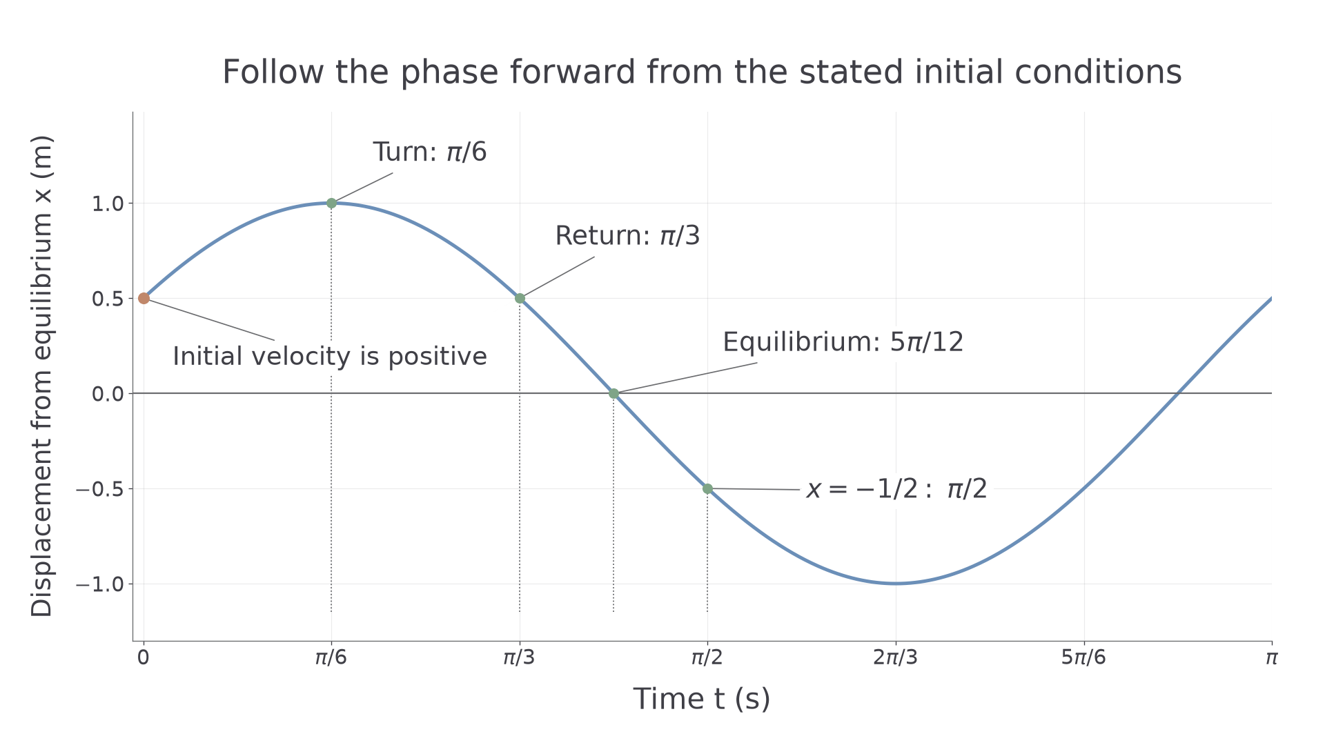
The positive starting velocity takes the particle to its positive extreme before its first equilibrium crossing

Worked example 5: first reaching equilibrium after an outward start

Question. For this motion, find the first positive time at equilibrium and the velocity then.

Plan. Move the phase forwards from $-\pi/3$ to the first subsequent cosine zero, $\pi/2$ .

2t-\frac\pi3=\frac\pi2 \Rightarrow t=\frac{5\pi}{12}\,\mathrm{s}

v=-2\sin(\pi/2)=-2\,\mathrm{m\,s^{-1}}

Why this step? The starting velocity is positive, so the particle first goes farther from equilibrium. The first equilibrium crossing occurs after its positive turning point, not a quarter-period after the stated start.

Answer. $t=5\pi/12\,\mathrm{s}$ , velocity $-2\,\mathrm{m\,s^{-1}}$ .

Check. The positive extreme occurs at $t=\pi/6$ , before this crossing. The speed at equilibrium is $a\omega=2$ , with negative direction on the returning branch.

Continue this lesson.

You’re previewing NovaLearn without an account. Create a free account to read the rest.

Create free account

Last Accessed

Core Pure Mathematics

Further Pure Mathematics 1

Further Pure Mathematics 2

Further Statistics 1

Further Statistics 2

Further Mechanics 1

Further Mechanics 2

Decision Mathematics 1

Decision Mathematics 2

FM2 4.2 - Simple harmonic motion of a particle

Prove SHM using displacement from equilibrium

Use motion data to identify the oscillation

Use the initial direction to choose the first event

Continue this lesson.

Learn faster with Nova