FP1 6.1 - Numerical solution of differential equations | Edexcel A-Level Further Mathematics

Replace derivatives by finite differences to approximate first- and second-order differential equations (FP1 6.1). You will use forward and central differences, generate solution values on a grid and distinguish starting-value calculations from boundary-value equations.

Three derivative approximations on a grid

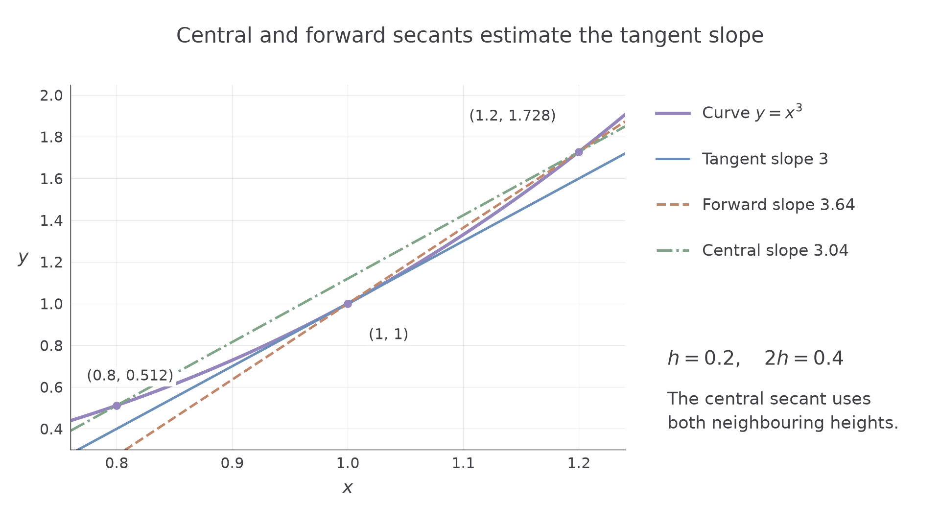
Can a table of heights stand in for a differential equation's derivatives? A forward secant estimates a tangent using the next height. A central secant uses heights on both sides, balancing their contributions.

Choose equally spaced points $x_n=x_0+nh$ , with $h>0$ . Write $y_n$ for the height associated with $x_n$ ; in a numerical solution these heights are themselves approximations. The subscripts label grid positions, rather than powers or derivatives.

You already know

An initial condition selects a solution curve, and a differential equation supplies gradients along that curve. A first-order initial-value problem normally gives one starting value; a second-order problem needs two pieces of data. A numerical approximation does not have to satisfy the equation exactly between grid points.

The difference of the two neighbouring secant gradients is

\frac{y_{n+1}-y_n}{h}-\frac{y_n-y_{n-1}}h =\frac{y_{n+1}-2y_n+y_{n-1}}h

Dividing that gradient change by the separation $h$ gives the second-difference estimate of the second derivative.

Forward, central and second differences

For an equally spaced grid, where $y$ is sufficiently smooth near the points used,

\left(\frac{\mathrm dy}{\mathrm dx}\right)_n \approx\frac{y_{n+1}-y_n}{h} \qquad\text{forward first difference}

\left(\frac{\mathrm dy}{\mathrm dx}\right)_n \approx\frac{y_{n+1}-y_{n-1}}{2h} \qquad\text{central first difference}

\left(\frac{\mathrm d^2y}{\mathrm dx^2}\right)_n \approx\frac{y_{n+1}-2y_n+y_{n-1}}{h^2} \qquad\text{central second difference}

The central first difference spans two grid intervals, while the second difference divides by $h^2$ .

Not in the formula booklet: learn it.

Central estimates require both neighbours, so they cannot be used at an endpoint without additional information.

Worked example 1: three estimates from one small table

Question. For $y=x^3$ , estimate $y'(1)$ by forward and central differences and $y''(1)$ by the second difference, using $h=0.1$ .

Plan. Find the three heights around $x=1$ , then use each approximation with its own denominator.

\begin{array}{c|ccc} x&0.9&1&1.1\\ \hline y&0.729&1&1.331 \end{array}

\begin{aligned} y'(1)_{\mathrm{forward}}&\approx\frac{1.331-1}{0.1}=3.31 && \text{one forward interval}\\ y'(1)_{\mathrm{central}}&\approx\frac{1.331-0.729}{0.2}=3.01 && \text{two intervals}\\ y''(1)&\approx\frac{1.331-2(1)+0.729}{0.01}=6 && \text{second difference} \end{aligned}

Why this step? The same three heights enter different expressions; a shared table does not mean the denominators are interchangeable.

Answer. The estimates are $3.31$ , $3.01$ and $6$ , respectively.

Check. The exact derivatives are $y'=3x^2$ , $y''=6x$ , giving $3$ and $6$ at $1$ . The central first estimate is closer here, and the second estimate is exact.

Change only the spacing to $h=0.05$ , keeping the function and centre fixed.

Worked example 2: halving the spacing

Question. Repeat the three estimates at $x=1$ using $h=0.05$ .

Plan. Recalculate the neighbouring heights; do not reuse those for the old grid.

\begin{array}{c|ccc} x&0.95&1&1.05\\ \hline y&0.857375&1&1.157625 \end{array}

\begin{aligned} y'(1)_{\mathrm{forward}}&\approx\frac{1.157625-1}{0.05}=3.1525 && \text{new forward spacing}\\ y'(1)_{\mathrm{central}}&\approx\frac{1.157625-0.857375}{0.1}=3.0025 && \text{span }2h\\ y''(1)&\approx\frac{1.157625-2+0.857375}{0.0025}=6 && \text{denominator }h^2 \end{aligned}

Why this step? Halving $h$ quarters $h^2$ , so the second-difference denominator must change by a different factor.

Answer. The estimates are $3.1525$ , $3.0025$ and $6$ .

Check. The central first-derivative error falls from $0.01$ to $0.0025$ . The second derivative remains exact.

There is a useful surprise: the central second difference is exact for every cubic polynomial, for any non-zero spacing when exact heights are used. Expanding the cubic at $x+h$ and $x-h$ cancels the odd powers of $h$ , leaving exactly its second derivative. This algebraic fact is not a separate booklet result. General smooth functions still produce approximation errors.

[DIAGRAM: asset_name: Forward and central secants around a tangent; asset_slug: 9fm0-fp1-difference-secants; caption: The central secant balances heights on both sides of the derivative point; description: A Cartesian graph of y equals x cubed near x equals 1 shows points at x equals 0.8, 1 and 1.2. A clay forward secant through x equals 1 and 1.2 has slope 3.64. A sage central secant through x equals 0.8 and 1.2 has slope 3.04. A blue tangent at x equals 1 has slope 3. The three lines have separate legend labels and the grid heights are marked.]
The central secant balances heights on both sides of the derivative point

Watch out

Smaller spacing usually reduces discretisation error for a smooth problem, but it also magnifies the effect of rounding in differences. Keep enough digits in stored heights, especially before division by $h^2$ .

Change the spacing to $0.2$ and keep the three denominators distinct.

Forward steps for a first-order equation

For $y'=f(x,y)$ , replacing the derivative by a forward difference gives an explicit update from the current point.

Rearrange $(y_{n+1}-y_n)/h\approx f(x_n,y_n)$ , then define the numerical scheme by the resulting update. Equality in that update describes the calculation, rather than an exact differential-equation solution.

Forward first-order update

For $y'=f(x,y)$ and grid $x_n=x_0+nh$ ,

y_{n+1}=y_n+h f(x_n,y_n)

Start from the given $y_0$ . The slope is evaluated at the current point, before moving to the next point. This is the forward Euler method.

Not in the formula booklet: learn it.

Use a table with separate columns for $x_n,y_n$ , the current slope and the next height. Retain working digits until the requested final rounding.

Worked example 3: two forward steps

Question. Use the forward-difference method with $h=0.1$ to estimate $y(0.2)$ , where $y'=x+y$ and $y(0)=1$ .

Plan. Use $y_{n+1}=y_n+0.1(x_n+y_n)$ , advancing $x_n$ and $y_n$ together.

\begin{aligned} y_1&=1+0.1(0+1)=1.1 && x_0=0\\ y_2&=1.1+0.1(0.1+1.1)=1.22 && x_1=0.1 \end{aligned}

Why this step? The second step uses the new height $1.1$ , not the original height $1$ , to estimate the slope at $x=0.1$ .

Answer. $y(0.2)\approx1.22$ .

Check. Two intervals of width $0.1$ reach $0.2$ . The exact function $2\mathrm e^x-x-1$ satisfies the problem and gives approximately $1.24281$ , so $1.22$ is an approximation rather than an exact value.

Change only the step length to $0.05$ , keeping the same initial-value problem and target point.

Worked example 4: more steps to the same target

Question. Repeat the estimate of $y(0.2)$ with $h=0.05$ .

Plan. Take four forward steps, using the current coordinates each time.

\begin{array}{c|c|c|c} n&x_n&y_n&x_n+y_n\\ \hline 0&0&1&1\\ 1&0.05&1.05&1.10\\ 2&0.10&1.105&1.205\\ 3&0.15&1.16525&1.31525 \end{array}

Thus

y_4=1.16525+0.05(1.31525)=1.2310125

Why this step? The target is unchanged, so halving the step doubles the required number of steps.

Answer. $y(0.2)\approx1.2310125$ , or $1.23101$ to six significant figures.

Check. This is closer to $1.24281$ than the previous estimate. That comparison concerns this problem; two numerical approximations alone would not prove an error bound.

A smooth exact solution is useful for checking a method in an example, but numerical methods remain useful when no manageable explicit solution is available.

Watch out

Wrong: use $y_{n+1}=y_n+hf(x_{n+1},y_n)$ for the forward update. That mixes the next horizontal coordinate with the current height. Right: evaluate the slope at the current pair $(x_n,y_n)$ , giving $y_{n+1}=y_n+hf(x_n,y_n)$ . Show the recurrence and intermediate values; a calculator's direct solution of the differential equation does not demonstrate the requested finite-difference method.

Take two larger steps for the next estimate.

Central first differences need two starting heights

A central first difference produces a two-step recurrence: its next height depends on both of the preceding stored heights.

For $y'=f(x,y)$ , substitute $(y_{n+1}-y_{n-1})/(2h)$ at $x_n$ , then rearrange.

Central first-order update

y_{n+1}=y_{n-1}+2h f(x_n,y_n),\qquad n\ge1

Two starting heights, $y_0,y_1$ , are needed. Use a supplied starting height or the instructed starting method, such as one forward step. The slope is still evaluated at the central point $(x_n,y_n)$ .

Not in the formula booklet: learn it.

The update jumps from the old height $y_{n-1}$ across two intervals. Adding $2hf$ to $y_n$ would use the wrong base height.

Continue this lesson.

You’re previewing NovaLearn without an account. Create a free account to read the rest.

Create free account

Last Accessed

Core Pure Mathematics

Further Pure Mathematics 1

Further Pure Mathematics 2

Further Statistics 1

Further Statistics 2

Further Mechanics 1

Further Mechanics 2

Decision Mathematics 1

Decision Mathematics 2

FP1 6.1 - Numerical solution of differential equations

Three derivative approximations on a grid

Forward steps for a first-order equation

Central first differences need two starting heights

Continue this lesson.

Learn faster with Nova