FS2 1.2 - Residuals and residual sum of squares
A fitted line needs checking as well as calculating. You will interpret signed residuals, calculate the residual sum of squares, use residual patterns to question a model, investigate possible outliers and compare fits on a consistent response scale.
Observed minus fitted gives a signed error
Can a model have residuals that add to zero and still miss a clear pattern in the data?
Yes. Positive and negative errors can cancel even when the model systematically misses a curve. To diagnose the fit, keep the individual residuals and their pattern, rather than looking only at their signed total.
You already know
The regression of a response on an explanatory variable minimises squared vertical residuals. For a fitted response , the residual is observed minus fitted: . Keep unrounded coefficients when calculating predictions and residuals.
Residuals have the same units as the response. A positive one means the observed response is larger than its fitted value; a negative one means it is smaller. The residual is a vertical difference, not a horizontal or perpendicular distance.
Worked example 1: an observation above the fitted model
Question. A time-height model is , with in seconds and in centimetres. An observation at height has time . Find and interpret its residual.
Plan. Predict time at the observed height, then subtract fitted time from observed time.
Why this step? Time is the response, so the residual compares times at the same observed height.
Answer. The residual is second. The observation took one second longer than the model predicts.
Check. The observed point lies above the fitted curve when time is on the vertical axis, agreeing with a positive residual.
Worked example 2 changes only the recorded time from to , at the same height.
Worked example 2: the sign reverses
Question. Find and interpret this second residual.
Plan. Retain fitted time and subtract it from the new observed time.
Why this step? The model and height have not changed, so the prediction stays fixed while the observation moves below it.
Answer. The residual is second; the observed time is one second less than predicted.
Check. Both examples have the same error magnitude and squared residual , while the signs distinguish their directions.
When coding has been used, calculate the prediction in the requested response units before subtracting. If a coefficient is rounded early, the final residual can lose accuracy even when the method is correct.
Watch out
Wrong: fitted minus observed, or the absolute difference when a residual is requested. Right: retain the sign in ; square only when the next calculation requires it.
Keep the observed time from Worked example 2 and change only the height to .
Measuring the total squared error
The residual sum of squares, or RSS, combines error sizes without allowing cancellation:
It is measured in squared response units. The signed sum of residuals can be zero while RSS is positive.
For an ordinary least squares line with an intercept, fitted to the observations being checked, the residuals sum to zero apart from rounding. This balance is a consequence of the fit, not evidence of perfect predictions, and is not printed as a separate booklet result.
Residual sum of squares of a least squares line
For the fitted regression of on , with ,
The booklet also gives , where the product moment correlation is defined. No derivation is required. These expressions apply to the least squares fit on these same data. In the formula booklet.
Do not apply this closed formula to an arbitrary proposed line. Its residuals can still be squared and added directly, but it need not achieve the least squares minimum.
Worked example 3: checking the formula against the residuals
Question. A dataset has
Its least squares line is . Find RSS using the summary formula and check it directly.
Plan. Calculate the centred sums, then compare with the sum of squared signed residuals.
Why this step? Square the cross-product before dividing; the numerator is not itself.
Answer. .
Check. The residuals are . They sum to zero, but their squared sum is
so the two methods agree.
Worked example 4 reflects every response using . The centred spread remains the same while the fitted association reverses.
Worked example 4: reversing the slope does not change squared error
Question. For the same -values, take responses . The fitted line is . Find RSS.
Plan. Use the new cross-product and retain the unchanged response sum of squares.
Why this step? Squaring removes the sign of . A negative slope is not inherently a worse fit than a positive one.
Answer. RSS is again .
Check. The new residuals are the negatives of the previous ones, so their squares are unchanged.
RSS is non-negative. A negative calculated value signals inconsistent summaries, a formula error or damaging rounding. If all responses are identical, the constant fitted line has RSS zero; correlation is then undefined, so use the direct or centred-sum formula rather than an undefined .
Watch out
Wrong: use the signed residual total, forget the square on , or round summaries before a subtraction of close values. Right: retain precision and check that RSS is at least zero.
Use another valid set of centred summaries.
Using the pattern to question the model
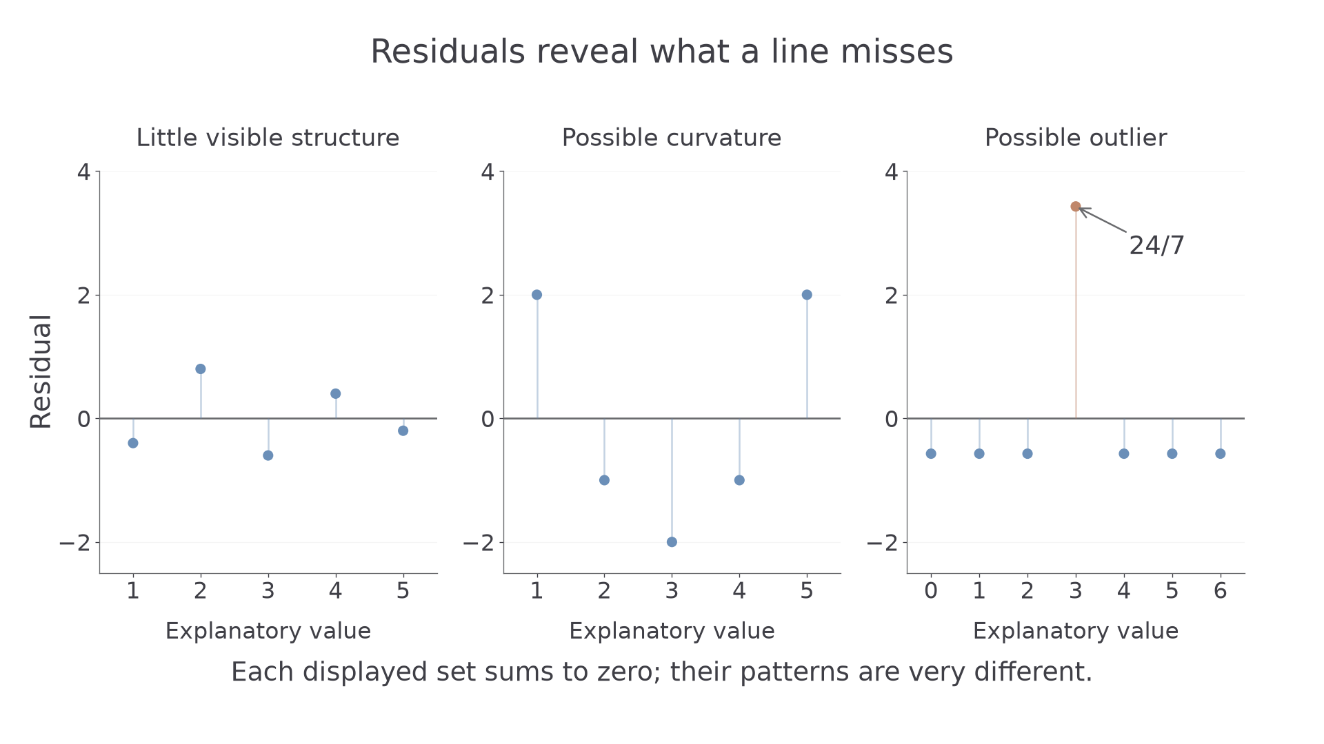
Plot residuals against the explanatory variable or fitted response, with a horizontal zero line. A reasonable linear mean relationship should not leave a clear curved pattern in those residuals.
A small dataset can show an accidental pattern, so residual plots suggest questions to investigate rather than prove a model true or false.
| Residual appearance | What to investigate |
|---|---|
| Scatter on both sides of zero with no obvious structure | The line may be a reasonable description; still check the context and data range. |
| Positive values at both ends and negative values in the middle | A curve may describe the mean relationship better than a line. |
| One residual much larger in magnitude than the others | A possible unusual observation or recording error; inspect it before changing the data. |
| A spread that increases with the explanatory value | Variation changes across the range; a single description of prediction uncertainty may be inadequate even if the mean is roughly linear. |
For example, the data , have least squares line . Their residuals are . The signed sum is zero, yet the clear U-shape reveals what the line misses.
[DIAGRAM: asset_name: Residual patterns reveal different model questions; asset_slug: 9fm0-fs2-119-residual-patterns; caption: A zero signed total cannot distinguish unstructured errors, curvature and a possible outlier; description: Three residual plots share a horizontal zero line. The first has residuals minus 0.4,0.8,minus 0.6,0.4,minus 0.2 at explanatory values one to five, with no obvious curve. The second has residuals 2,minus 1,minus 2,minus 1,2 at one to five and is labelled possible curvature. The third has six residuals minus four sevenths and one residual twenty-four sevenths at the central explanatory value three, and is labelled possible outlier. A note says each displayed residual set sums to zero]
Continue this lesson.
You’re previewing NovaLearn without an account. Create a free account to read the rest.
Create free account