FP1 3.2 - Solving differential equations by substitution | Edexcel A-Level Further Mathematics

Use a given substitution to turn an unfamiliar differential equation into a first-order linear or constant-coefficient second-order equation (FP1 3.2). You will transform derivatives and initial conditions, solve using Core Pure methods and return to the original variables with the correct domain.

Changing the dependent variable

How can a perfectly smooth transformed solution produce a vertical asymptote in the original solution? A substitution can simplify an equation while making a particular transformed value forbidden. Solving the new equation is only part of the job.

A given substitution tells you the relationship between the old and new variables. Differentiate that relationship before replacing terms in the equation. State where the relationship is valid, and keep that restriction when you change back.

You already know

The chain and product rules connect derivatives of related functions. Core Pure supplies integrating factors for first-order linear equations, and complementary functions plus particular integrals for constant-coefficient second-order equations. Apply initial conditions to the complete solution.

Consider the nonlinear equation $y'=y+y^2$ . For $y\ne0$ , the substitution $u=1/y$ gives

\begin{aligned} u'&=-\frac{y'}{y^2} && \text{differentiate the reciprocal}\\ &=-\frac{y+y^2}{y^2}=-u-1 && \text{use the original equation} \end{aligned}

Thus $u'+u=-1$ , a first-order linear equation. These substitution and transformation results are not supplied in the formula booklet; derive them from the given relationship.

Recovering the original solution

For the given substitution $u=1/y$ , on an interval where $y\ne0$ ,

u'= -\frac{y'}{y^2},\qquad y=\frac1u

Recover $y$ only where $u\ne0$ . If the substitution excludes a possible original solution, check that solution directly in the original equation.

Not in the formula booklet: learn it.

Here $y=0$ is an original solution, but cannot be represented by $u=1/y$ . It must be considered separately if the original question asks for all solutions. Our positive initial values exclude it from the initial-value problems below.

Worked example 1: a reciprocal makes the equation linear

Question. Use $u=1/y$ to solve $y'=y+y^2$ , with $y(0)=1$ . State the largest interval containing zero on which this solution is defined.

Plan. Transform the equation and initial value, use an integrating factor for $u$ , then exclude zeros of $u$ when recovering $y$ .

\begin{aligned} u'+u&=-1 && \text{reciprocal transformation}\\ u(0)&=1 && u=1/y\\ \frac{\mathrm d}{\mathrm dx}(\mathrm e^x u)&=-\mathrm e^x && \text{integrating factor }\mathrm e^x\\ \mathrm e^xu&=-\mathrm e^x+C && \text{integrate}\\ u&=C\mathrm e^{-x}-1 && \text{divide by }\mathrm e^x\\ 1&=C-1\quad\Rightarrow\quad C=2 && \text{transformed initial value} \end{aligned}

Therefore

y=\frac1{2\mathrm e^{-x}-1}

The denominator is zero at $x=\ln2$ . The connected interval containing $0$ is $x<\ln2$ .

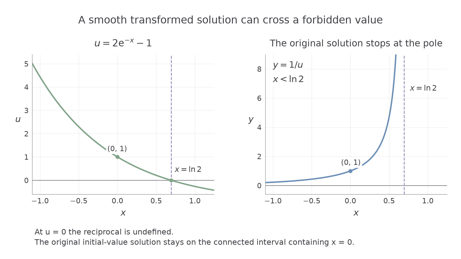
Why this step? A solution of the transformed equation can pass through $u=0$ , but its reciprocal cannot; the original initial-value solution stops at that point.

Answer. $y=1/(2\mathrm e^{-x}-1)$ , for $-\infty<x<\ln2$ .

Check. Put $D=2\mathrm e^{-x}-1$ . Then $y'=(D+1)/D^2=1/D+1/D^2=y+y^2$ , and $y(0)=1$ .

Change only the initial value from $1$ to $2$ . The transformed equation stays the same, but the constant and the location of the pole change.

Worked example 2: the initial condition changes the endpoint

Question. Use the same substitution to solve $y'=y+y^2$ , with $y(0)=2$ , on its largest interval containing zero.

Plan. Reuse the transformed general solution and apply the reciprocal initial value $u(0)=1/2$ .

\begin{aligned} u&=C\mathrm e^{-x}-1 && \text{solution of }u'+u=-1\\ \frac12&=C-1\quad\Rightarrow\quad C=\frac32 && \text{new initial value}\\ y&=\frac1{\frac32\mathrm e^{-x}-1} && \text{return to }y\\ \frac32\mathrm e^{-x}-1&=0\quad\Rightarrow\quad x=\ln\frac32 && \text{excluded endpoint} \end{aligned}

Why this step? Transforming $y(0)=2$ into $u(0)=2$ would solve a different initial-value problem; the point's independent coordinate stays zero, while the dependent value is reciprocated.

Answer. $y=1/(\frac32\mathrm e^{-x}-1)$ , for $x<\ln(3/2)$ .

Check. At zero the denominator is $1/2$ , giving $y(0)=2$ . Writing $D=\frac32\mathrm e^{-x}-1$ again gives $y'=(D+1)/D^2=y+y^2$ .

There is a surprising consequence: $u=2\mathrm e^{-x}-1$ is smooth for every real $x$ , yet its reciprocal becomes arbitrarily large as $x$ approaches $\ln2$ from below. The finite endpoint comes from the inverse substitution, rather than a failure of the linear equation's solution.

[DIAGRAM: asset_name: A reciprocal substitution and its forbidden value; asset_slug: 9fm0-fp1-reciprocal-domain; caption: The transformed solution crosses zero where the original solution has a pole; description: Two Cartesian panels share the independent variable x. The left shows u equals 2 exp of minus x minus 1, passing through (0,1) and crossing zero at ln 2. The right shows y equals its reciprocal only on x less than ln 2, passing through (0,1) and increasing without bound at the dashed vertical line x equals ln 2. Clear labels distinguish the valid initial-value interval from the transformed solution's wider domain.]
The transformed solution crosses zero where the original solution has a pole

Watch out

Wrong: giving every real $x$ as the domain just because $u$ is defined there. Right: impose the inverse substitution's restrictions and choose the connected interval containing the initial point. Here the separate equilibrium $y=-1$ is included by $C=0$ , while $y=0$ was excluded by the substitution.

Vary the initial value again, and carry its effect through to the endpoint.

Changing the independent variable

A substitution for the independent variable changes what a prime means. Use distinct notation until the derivative conversion is complete.

For $x>0$ , suppose the given substitution is $t=\ln x$ , and define $Y(t)=y(\mathrm e^t)$ . Here $y'$ means differentiation with respect to $x$ , while $Y'$ means differentiation with respect to $t$ . Since $\mathrm dt/\mathrm dx=1/x$ , the chain rule gives

\begin{aligned} y'&=\frac{Y'}x\\ y''&=\frac{\mathrm d}{\mathrm dx}\left(\frac{Y'}x\right) =\frac{Y''-Y'}{x^2} \end{aligned}

Consequently,

x^2y''+xy'-y=Y''-Y

The variable coefficients have disappeared. This particular transformation is not printed in the formula booklet.

Initial data after $t=\ln x$

For $x=a>0$ , with $Y(t)=y(\mathrm e^t)$ ,

Y(\ln a)=y(a),\qquad Y'(\ln a)=a y'(a)

The first derivative condition changes because $Y'=xy'$ . Recover $y(x)$ by putting $t=\ln x$ .

Not in the formula booklet: learn it.

At $x=1$ , the new centre is $t=0$ , and the factor $a$ happens to equal one. That simplification does not hold at a general initial point.

Worked example 3: a logarithm removes variable coefficients

Question. For $x>0$ , solve

x^2y''+xy'-y=0,\qquad y(1)=2,\quad y'(1)=0

using the substitution $t=\ln x$ .

Plan. Convert to a constant-coefficient equation for $Y(t)$ , transform both initial conditions and use the auxiliary equation.

\begin{aligned} Y''-Y&=0 && \text{converted equation}\\ m^2-1&=0\quad\Rightarrow\quad m=1,-1 && \text{auxiliary equation}\\ Y&=A\mathrm e^t+B\mathrm e^{-t} && \text{complementary function}\\ Y(0)&=2,\qquad Y'(0)=0 && x=1\ \text{means }t=0\\ A+B&=2,\qquad A-B=0 && \text{apply both conditions}\\ A&=B=1 \end{aligned}

Returning to $x$ , $\mathrm e^t=x$ and $\mathrm e^{-t}=1/x$ .

Why this step? The constant-coefficient equation is solved in $t$ ; leaving $\mathrm e^t$ in the final expression would leave the original problem unfinished.

Answer. $y=x+1/x$ , for $x>0$ .

Check. $y'=1-x^{-2}$ , $y''=2x^{-3}$ , so $x^2y''+xy'-y=2/x+x-1/x-x-1/x=0$ . The value and slope at $1$ are $2$ and $0$ .

Continue this lesson.

You’re previewing NovaLearn without an account. Create a free account to read the rest.

Create free account

Last Accessed

Core Pure Mathematics

Further Pure Mathematics 1

Further Pure Mathematics 2

Further Statistics 1

Further Statistics 2

Further Mechanics 1

Further Mechanics 2

Decision Mathematics 1

Decision Mathematics 2

FP1 3.2 - Solving differential equations by substitution

Changing the dependent variable

Changing the independent variable

Continue this lesson.

Learn faster with Nova