FS1 3.1 - Geometric and negative binomial probabilities | Edexcel A-Level Further Mathematics

Some experiments stop when a success arrives, rather than after a fixed number of trials. You will model the trial of the first or a later success, calculate exact and cumulative probabilities, and see why a long run of failures does not make the next success more likely under an independent-trials model.

The trial of the first success

After nine unsuccessful attempts, have you earned a better chance on the next attempt? Keep that question in mind while building the waiting-time model.

Suppose independent trials each have success probability $p=0.3$ . A first success on trial $5$ requires the exact pattern $FFFFS$ : four failures followed by a success. Its probability is $0.7^4(0.3)$ . Here “success” means the event being counted; it could even be a fault.

You already know

A discrete model needs a precise variable definition, possible values and probabilities. Independent events have probabilities that multiply. All probabilities must be non-negative and sum to $1$ .

For a geometric model, trials are independent, each has two labelled outcomes, and the success probability stays constant. Sampling without replacement, fatigue or learning may break those assumptions.

Geometric distribution

If $X$ counts the trial on which the first success occurs in independent trials with constant probability $p$ , write $X\sim\operatorname{Geo}(p)$ . Pearson counts the successful trial, so $X=1,2,3,\ldots$ . The number of failures is $X-1$ , which starts at $0$ ; do not confuse the conventions.

For $0<p<1$ , reaching trial $x$ means exactly $x-1$ failures precede its success.

Geometric probability

For $X\sim\operatorname{Geo}(p)$ , $0<p<1$ ,

\mathrm P(X=x)=p(1-p)^{x-1},\qquad x=1,2,3,\ldots

In the formula booklet.

At $p=1$ , $X=1$ with certainty. The value $p=0$ gives no finite success time and is excluded. For $0<p<1$ , the infinite probabilities add to $p/(1-(1-p))=1$ , using the geometric-series sum.

Worked example 1: one final success

Question. Independent trials have success probability $0.3$ . Find the probability that the first success is on trial $5$ .

Plan. Require four failures, then one success.

\begin{aligned} X&\sim\operatorname{Geo}(0.3) && \text{trial of the first success} \\ \mathrm P(X=5)&=(0.7)^4(0.3) && FFFFS \\ &=0.07203 && \text{multiply probabilities} \end{aligned}

Why this step? There is only one permitted pattern: an earlier success would stop the experiment before trial $5$ .

Answer. $0.0720$ to $3$ significant figures.

Check. This is less than $0.3$ , since four earlier failures are also required.

Worked example 2 changes only the required trial, from $5$ to $6$ , adding one failure.

Worked example 2: one additional failure

Question. For the same trials, find the probability that the first success is on trial $6$ .

Plan. Use five failures followed by a success.

\begin{aligned} \mathrm P(X=6)&=(0.7)^5(0.3) && FFFFFS \\ &=0.050421 && \text{evaluate without early rounding} \end{aligned}

Why this step? One extra failure multiplies the previous probability by $0.7$ ; the final success probability stays fixed.

Answer. $0.0504$ to $3$ significant figures.

Check. $0.050421/0.07203=0.7$ , the extra failure factor.

That constant ratio shows that geometric probabilities decrease with each additional trial when $0<p<1$ .

Watch out

Wrong: $\mathrm P(X=6)=p(1-p)^6$ . That counts six failures before success on trial $7$ . Right: the exponent is $6-1$ , since $X$ includes the successful trial.

Add one more failure in your turn.

Tails, intervals and a trial limit

Waiting longer than a trial limit means that every trial so far has failed.

Write $q=1-p$ . The event $X>n$ means no success in the first $n$ trials, giving $q^n$ . Its complement gives success by trial $n$ . Since $X$ is integer-valued, $X\ge n$ instead requires failures in only the first $n-1$ trials.

Geometric tails and cumulative probabilities

For $0<p<1$ , $q=1-p$ , and positive integer $n$ :

\mathrm P(X>n)=q^n,\qquad \mathrm P(X\ge n)=q^{n-1},\qquad \mathrm P(X\le n)=1-q^n

For integers $0\le a<b$ , $\mathrm P(a<X\le b)=q^a-q^b$ . These consequences of the supplied probability formula are not printed explicitly. Not in the formula booklet: learn it.

“At least”, “more than” and “by” place the endpoint differently. Write the event before calculating.

Worked example 3: success by a fixed limit

Question. For independent trials with success probability $0.3$ , find the probability of at least one success by trial $8$ .

Plan. Subtract eight consecutive failures from $1$ .

\begin{aligned} \mathrm P(X\le8)&=1-\mathrm P(X>8) && \text{complement} \\ &=1-(0.7)^8 && \text{eight failures} \\ &=0.94235199 && \text{evaluate} \end{aligned}

Why this step? The complement contains no success at all, rather than a success at one particular time.

Answer. $0.942$ to $3$ significant figures.

Check. The remaining tail is $0.05764801$ ; the two probabilities sum to $1$ .

Worked example 4 changes the fixed trial limit into a quantity to choose: require a success probability of at least $0.95$ .

Worked example 4: choosing the minimum trial limit

Question. Find the least integer $n$ for which $\mathrm P(X\le n)\ge0.95$ , when $X\sim\operatorname{Geo}(0.3)$ .

Plan. Rearrange the cumulative probability, take logarithms and check neighbouring integers.

\begin{aligned} 1-(0.7)^n&\ge0.95 && \text{required probability} \\ (0.7)^n&\le0.05 && \text{failure tail} \\ n\ln0.7&\le\ln0.05 && \text{take logarithms} \\ n&\ge\frac{\ln0.05}{\ln0.7}=8.399\ldots && \ln0.7<0 \end{aligned}

Why this step? Dividing by negative $\ln0.7$ reverses the inequality. The least allowable integer is above the real bound.

Answer. $n=9$ .

Check. $1-0.7^8=0.94235199<0.95$ , while $1-0.7^9=0.959646393\ge0.95$ .

For an interval, subtract tails with their endpoints intact: $\mathrm P(3<X\le6)=0.7^3-0.7^6$ , which includes first successes on trials $4,5,6$ .

Watch out

Wrong: $\mathrm P(X\ge n)=q^n$ . Right: $q^{n-1}$ , because success may occur on trial $n$ . Test the boundary $\mathrm P(X\ge1)=1$ .

Increase the required cumulative probability in the next problem.

The trial of the rth success

For a specified later success, the last trial is still fixed as a success, but earlier successes can be arranged in several ways.

For a third success on trial $6$ , the first five trials contain exactly two successes and three failures. There are $\binom52=10$ arrangements of those first five trials; the sixth trial must then succeed. Every allowed full pattern has three successes and three failures.

[DIAGRAM: asset_name: Ten ways to get the third success on trial six; asset_slug: 9fm0-fs1-106-last-success; caption: Rearrange the first five trials and keep the final success fixed; description: A table of ten exact outcome sequences lists every choice of two success positions among the first five trials, followed by a fixed sixth-trial success. S cells are pale clay and F cells pale blue. Headers identify trials 1 to 6, the last column is outlined, and a side panel explains that only the first five positions can be rearranged]
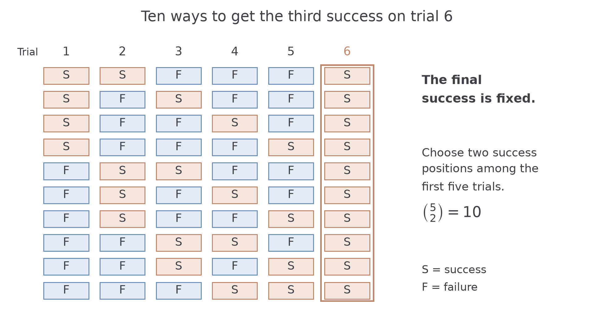
Rearrange the first five trials and keep the final success fixed

The same reasoning works for any positive integer target $r$ .

Negative binomial waiting time

Let $T$ count the trial on which success number $r$ occurs, in independent trials with constant success probability $p$ . Write $T\sim\operatorname{NB}(r,p)$ , with support $r,r+1,r+2,\ldots$ . Pearson counts all trials, including the $r$ successes. The number of failures is $T-r$ , starting at zero. The case $r=1$ is geometric.

Continue this lesson.

You’re previewing NovaLearn without an account. Create a free account to read the rest.

Create free account

Last Accessed

Core Pure Mathematics

Further Pure Mathematics 1

Further Pure Mathematics 2

Further Statistics 1

Further Statistics 2

Further Mechanics 1

Further Mechanics 2

Decision Mathematics 1

Decision Mathematics 2

FS1 3.1 - Geometric and negative binomial probabilities

The trial of the first success

Tails, intervals and a trial limit

The trial of the rth success

Continue this lesson.

Learn faster with Nova