FS1 6.1 - Goodness of fit tests | Edexcel A-Level Further Mathematics

A model predicts a whole pattern of frequencies, not just a mean. You will compare observed and expected counts using a chi-squared goodness of fit test, pool small expected cells and adjust the degrees of freedom when parameters are estimated from the data.

Measuring the discrepancy from a model

Is an excess of five observations equally surprising when a model expected five and when it expected fifty?

No. The chi-squared contribution is $5^2/5=5$ in the first case, but $5^2/50=0.5$ in the second. The same numerical discrepancy receives ten times as much weight against the smaller expectation. A goodness of fit test combines these scaled discrepancies across all categories.

You already know

A model assigns probabilities that are non-negative and sum to $1$ . Earlier FS1 lessons supply binomial, Poisson and geometric probabilities and their parameter conditions. A null hypothesis describes the population model being tested; an observed sample does not have to match its expectations exactly.

The categories must be mutually exclusive and cover every possible outcome. For an unbounded count, a final category such as “at least $4$ ” includes the entire remaining tail.

Observed and expected frequencies

An observed frequency $O_i$ is the number of sample observations in category $i$ . Its expected frequency $E_i$ is the count predicted by the null model for that same sample size. Expected frequencies need not be integers.

If each observation has null probability $p_i$ of falling in a category, multiply by the number sampled.

Expected category frequencies

For $N$ independent observations classified into exhaustive categories with null probabilities $p_1,\ldots,p_k$ ,

E_i=Np_i,\qquad \sum_{i=1}^k E_i=N

Retain unrounded expected frequencies in later calculations. Not in the formula booklet: learn it.

Squaring the discrepancies prevents positive and negative differences from cancelling. Dividing by their expectations makes the comparison sensitive to the model's predicted scale.

Chi-squared discrepancy statistic

For the categories retained in the test, with $E_i>0$ ,

T=\sum_{i=1}^k\frac{(O_i-E_i)^2}{E_i}

Under a suitable null model, $T$ has an approximate chi-squared distribution with the appropriate degrees of freedom. Its approximation requires sufficiently large expected frequencies. In the formula booklet.

The statistic is non-negative and is zero only when every retained observed count equals its expectation. A large value indicates poor agreement. If the null gives a category probability zero but that category is observed, the proposed model is already contradicted; do not divide by zero in this formula.

Worked example 1: a discrete uniform model

Question. A spinner has four labelled outcomes. In $100$ independent spins the counts are $40,25,20,15$ . Assuming a discrete uniform model, find the expected frequencies and $T$ .

Plan. Equal outcome probabilities give equal expectations; calculate all four contributions.

\begin{aligned} p_i&=\frac14,\qquad E_i=100\left(\frac14\right)=25 &&\text{each of the four outcomes}\\ T&=\frac{(40-25)^2}{25} +\frac{(25-25)^2}{25} +\frac{(20-25)^2}{25} +\frac{(15-25)^2}{25} &&\text{use every category}\\ &=9+0+1+4=14 &&\text{sum scaled squared differences} \end{aligned}

Why this step? Subtracting raw discrepancies would give zero because both sets total $100$ . Their squares measure disagreement instead.

Answer. All four expected frequencies are $25$ , and $T=14$ .

Check. The expectations total $100$ , and every contribution is non-negative.

Worked example 2 changes only the observed counts, bringing them closer to the same null expectations.

Worked example 2: closer agreement

Question. Repeat the calculation if the counts are $30,25,25,20$ .

Plan. Keep all expected frequencies at $25$ .

\begin{aligned} T&=\frac{(30-25)^2}{25} +\frac{(25-25)^2}{25} +\frac{(25-25)^2}{25} +\frac{(20-25)^2}{25}\\ &=1+0+0+1=2 \end{aligned}

Why this step? Expectations come from the null probabilities and sample size, not by adjusting them to resemble the observed counts.

Answer. $T=2$ .

Check. A smaller discrepancy produces a smaller statistic. Whether either value is significant also depends on the degrees of freedom and significance level.

Use counts, rather than percentages substituted as though they were observations.

Watch out

Wrong: use $(O-E)^2/O$ , round expected counts to whole numbers, or omit a tail category. Right: divide by $E$ , retain precision and check that both frequency totals equal the sample size.

Move the two outer counts again while preserving the total.

Completing a test for a specified distribution

The null hypothesis states the proposed distribution, including fixed parameter values. The alternative says that this distribution is not a suitable model. This is a test of the whole frequency pattern, rather than a one-sided test of a single mean.

With $k$ retained categories and all model parameters specified independently of the sample, the degrees of freedom are $\nu=k-1$ . One constraint comes from the fixed total: after $k-1$ counts are chosen, the last is determined. This degrees-of-freedom rule is not printed in the booklet.

Right-tail chi-squared decision

Under $H_0$ , use $T$ approximately distributed as $\chi^2_\nu$ . At level $\alpha$ , either:

\text{reject if }T>c,\quad \mathrm P(\chi^2_\nu>c)=\alpha

or calculate the upper-tail p-value

p_{\text{value}}=\mathrm P(\chi^2_\nu\ge T_{\text{observed}})

and reject when it is at most $\alpha$ . The chi-squared model is continuous, so a single boundary point has probability zero. The critical-value tables are supplied; the decision rule is not. Not in the formula booklet: learn it.

Both excesses and shortages increase $T$ , so goodness of fit uses the upper chi-squared tail. Do not split a $5\%$ significance level into two $2.5\%$ tails. The booklet table headings are upper-tail probabilities; quote a tabulated critical value in full. A calculator may instead give the corresponding upper-tail p-value.

Worked example 3: testing a binomial model

Question. The counts of successes in $80$ independent three-trial experiments are:

Successes	$0$	$1$	$2$	$3$
Observed	$8$	$32$	$28$	$12$

Test at the $5\%$ level whether $\mathrm B(3,0.5)$ is a suitable model.

Plan. Obtain the four binomial probabilities, check expectations, then compare with $\chi^2_3$ .

\begin{aligned} H_0&:\ X\sim\mathrm B(3,0.5),\qquad H_1:\ \text{this model is not suitable}\\ (p_0,p_1,p_2,p_3)&=\left(\frac18,\frac38,\frac38,\frac18\right) &&\text{specified binomial probabilities}\\ (E_0,E_1,E_2,E_3)&=(10,30,30,10) &&80\text{ times each probability}\\ T&=\frac4{10}+\frac4{30}+\frac4{30}+\frac4{10} =1.066666\ldots &&\text{all expectations at least }5\\ \nu&=4-1=3,\qquad c=7.815 &&5\%\text{ upper-tail critical value} \end{aligned}

Why this step? The parameters $3$ and $0.5$ were specified, so no parameter has been estimated from these counts.

Answer. $1.066666\ldots<7.815$ , so do not reject $H_0$ . There is insufficient evidence at the $5\%$ level that the binomial model is unsuitable.

Check. A calculator gives upper-tail p-value $0.7851263\ldots>0.05$ , agreeing with the critical-value decision.

Worked example 4 changes only the observed counts. The null probabilities, sample size, degrees of freedom and critical value remain the same.

Worked example 4: stronger disagreement

Question. Repeat the test if the observed counts are $4,24,36,16$ .

Plan. Keep expectations $10,30,30,10$ and recalculate $T$ .

\begin{aligned} T&=\frac{(-6)^2}{10}+\frac{(-6)^2}{30} +\frac{6^2}{30}+\frac{6^2}{10}\\ &=3.6+1.2+1.2+3.6=9.6\\ \nu&=3,\qquad 9.6>7.815 &&\text{same }5\%\text{ comparison} \end{aligned}

Why this step? Changing the data changes the statistic, not a fixed null model's expectations.

Answer. Reject $H_0$ . There is sufficient evidence that $\mathrm B(3,0.5)$ is not a suitable model for the experiment counts.

Check. The upper-tail p-value is $0.0222909\ldots<0.05$ .

The diagram places the statistic and critical value in the same upper-tail comparison.

[DIAGRAM: asset_name: The upper tail detects poor fit; asset_slug: 9fm0-fs1-111-chi-tail; caption: Large discrepancies fall in the upper tail of the approximate chi-squared reference distribution; description: A chi-squared density curve with three degrees of freedom has the region above the five per cent critical value 7.815 shaded pale clay. A dashed line marks 7.815 and a separate labelled arrow marks the observed statistic 9.6 within the rejection region. The curve is labelled as the approximate null reference distribution, and the shaded area is labelled 0.05]
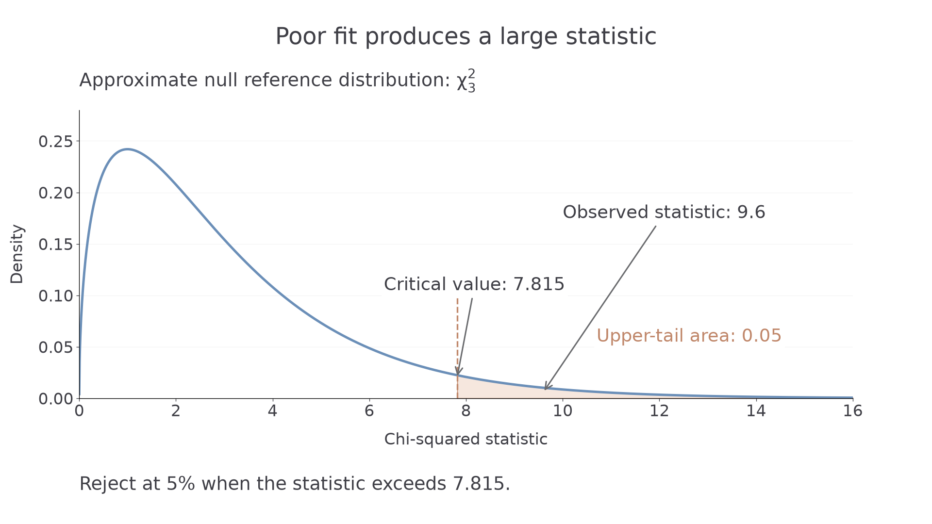
Large discrepancies fall in the upper tail of the approximate chi-squared reference distribution

Not rejecting a model does not prove it true. The sample may simply lack evidence against it; a goodness of fit test also does not establish the independence of the underlying observations.

Watch out

Wrong: reject when $T<c$ , or split the stated level between two chi-squared tails. Both excesses and shortages already increase the squared-discrepancy statistic, so large $T$ indicates poor fit. Right: use the upper tail and reject when $T>c$ at the stated level; otherwise give an insufficient-evidence conclusion.

The comparison then needs a complete contextual conclusion.

Exam tip

State both hypotheses, the retained categories and expectations, the statistic, degrees of freedom, critical value or p-value, and a conclusion about the proposed model in context.

The final variation lies between the two example datasets.

Continue this lesson.

You’re previewing NovaLearn without an account. Create a free account to read the rest.

Create free account

Last Accessed

Core Pure Mathematics

Further Pure Mathematics 1

Further Pure Mathematics 2

Further Statistics 1

Further Statistics 2

Further Mechanics 1

Further Mechanics 2

Decision Mathematics 1

Decision Mathematics 2

FS1 6.1 - Goodness of fit tests

Measuring the discrepancy from a model

Completing a test for a specified distribution

Continue this lesson.

Learn faster with Nova