D2 1.2 - Stepping-stone method and improvement indices | Edexcel A-Level Further Mathematics

You will calculate shadow costs and improvement indices, make stepping-stone improvements with explicit entering and exiting cells, recognise optimality, and handle degenerate and unbalanced transportation problems.

Shadow costs and the sign of an improvement

Can two different sets of shadow costs describe exactly the same shipments and total cost? Yes: a degenerate solution can have different valid choices of zero basic cell. First learn what the numbers measure and how they guide an improvement.

You already know

A feasible transportation allocation meets each supply and demand, with non-negative quantities. North-west corner supplies a starting allocation. Total cost multiplies each allocated quantity by its unit cost.

Use the following unit costs, with supplies $20,25,30$ and demands $15,35,25$ :

	$P$	$Q$	$R$
$A$	$8$	$6$	$10$
$B$	$9$	$7$	$4$
$C$	$3$	$4$	$2$

The starting non-zero allocations are $AP=15,AQ=5,BQ=25,CQ=5,CR=25$ , of cost $395$ pounds. These five cells are basic. An empty non-basic cell is a candidate to enter the allocation.

Pearson shadow costs and improvement indices

For a basic cell with unit cost $C_{ij}$ , choose row shadow costs $R_i$ and column shadow costs $K_j$ satisfying

R_i+K_j=C_{ij}

Set the first row shadow cost to zero to begin. For each non-basic cell, calculate

I_{ij}=C_{ij}-R_i-K_j

This is the cost change per extra unit sent around its valid adjustment cycle. For a minimisation problem, a negative index is an improving direction; choose a most negative index unless an entering cell is specified.

Not in the formula booklet: learn it.

Use unit costs, not allocated quantities, in these equations. Shadow costs can be negative even when every actual shipping cost is positive. They are computational row and column values, not extra charges added to the bill.

Worked example 1: calculate every index

Question. Find the shadow costs and improvement indices for the starting allocation. State an entering cell.

Plan. Set $R_A=0$ , use each basic cell to determine the remaining row and column values, then test every non-basic cell.

\begin{aligned} K_P&=8 &&\text{from }AP\\ K_Q&=6 &&\text{from }AQ\\ R_B&=7-6=1 &&\text{from }BQ\\ R_C&=4-6=-2 &&\text{from }CQ\\ K_R&=2-(-2)=4 &&\text{from }CR \end{aligned}

Non-basic cell	Index calculation	Index
$AR$	$10-0-4$	$6$
$BP$	$9-1-8$	$0$
$BR$	$4-1-4$	$-1$
$CP$	$3-(-2)-8$	$-3$

Why choose $CP$ , not the cost- $2$ cell $CR$ ? $CR$ is already basic; entering choices are made by non-basic improvement indices, not the smallest unit cost.

Answer. Row shadows are $0,1,-2$ ; column shadows are $8,6,4$ . Choose $CP$ , with most negative index $-3$ .

Check. Every basic cell satisfies its cost equation, including $R_C+K_R=-2+4=2$ .

Worked example 2 changes only the non-basic unit cost $CP$ , from $3$ to $4$ .

Worked example 2: changing a non-basic cost

Question. Recalculate the shadows, indices and entering choice when $C_{CP}=4$ , retaining the same allocation.

Plan. The basic costs have not changed, so retain their shadow equations and update the affected index.

The shadows remain

(R_A,R_B,R_C)=(0,1,-2),\qquad(K_P,K_Q,K_R)=(8,6,4)

The indices are

I_{AR}=6,\quad I_{BP}=0,\quad I_{BR}=-1,\quad I_{CP}=4-(-2)-8=-2

Why do the shadow costs stay fixed? They are determined by basic-cell costs; the altered cell is currently non-basic.

Answer. $CP$ remains the entering choice, now with index $-2$ .

Check. Its index increased by exactly one, matching the one-pound increase in that unit cost.

[DIAGRAM: asset_name: Shadow costs around an improvement-index table; asset_slug: 9fm0-d2-181-shadow-indices; caption: For the cost-3 CP case, a basic cell is marked X and every other entry is an improvement index.; description: Pearson-style table with row shadow costs0,1,-2 and column shadows8,6,4; body cells AP,AQ,BQ,CQ,CR marked X, and AR6,BP0,BR-1,CP-3.]

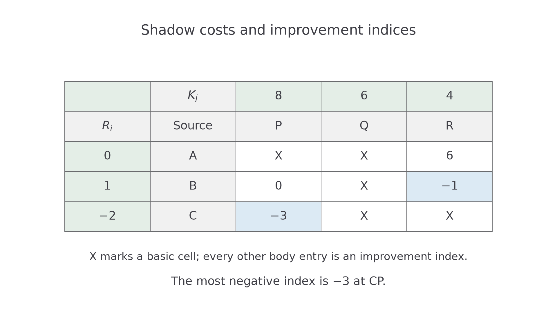
If indices tie for most negative, either tied cell may be chosen unless the question specifies one. State the choice so the next route can be checked.

Watch out

Wrong: calculate $R_i+K_j-C_{ij}$ , or use shipment quantities in the shadow equations. Right: use $I_{ij}=C_{ij}-R_i-K_j$ ; negative means a possible cost reduction.

Raise the same non-basic cost once more.

The route, adjustment amount and exiting cell

Adding stock to one cell alone would upset its row and column totals. Instead, use a closed route of horizontal and vertical moves, alternating additions and subtractions at its corner cells.

Stepping-stone adjustment

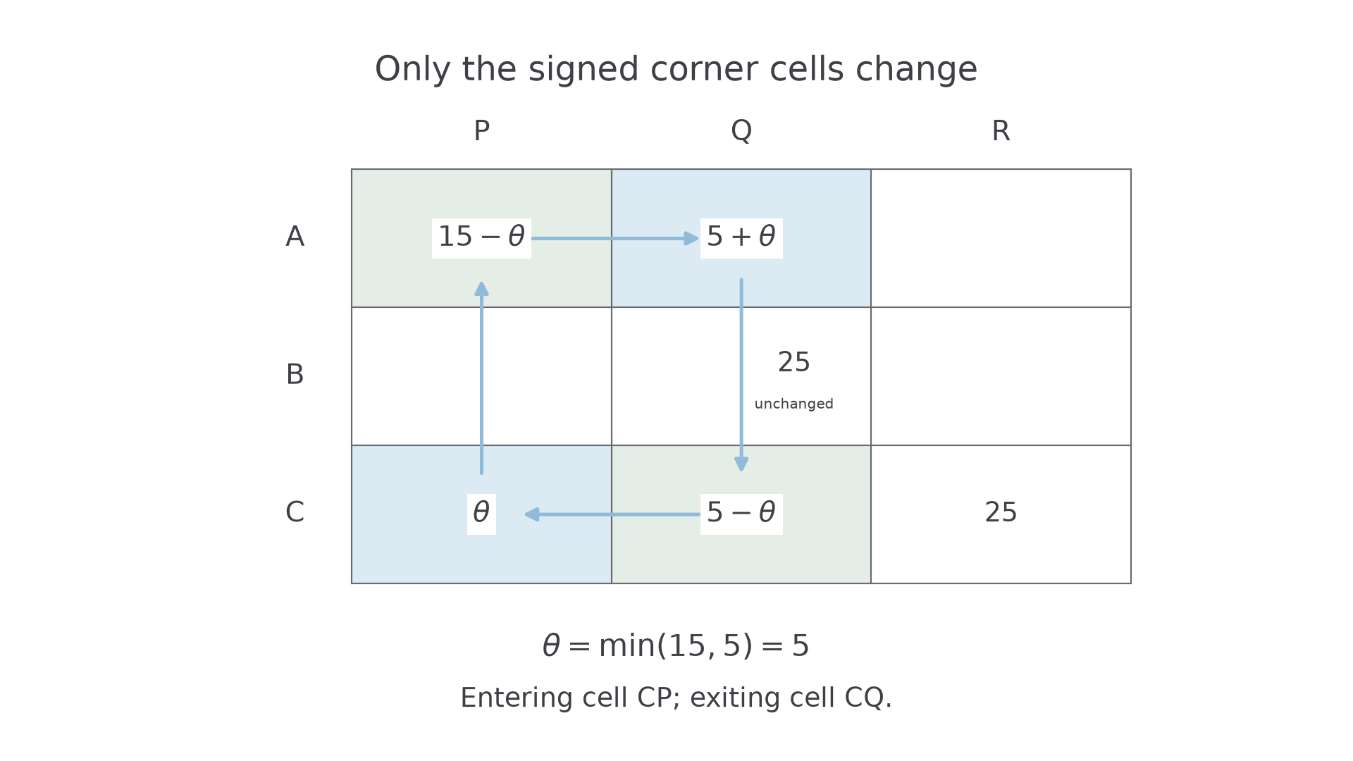
Start at the non-basic entering cell with $+\theta$ . Form a closed horizontal-and-vertical route whose other corner cells are basic, alternating $-\theta,+\theta,-\theta,\ldots$ . The entering cell is the only non-basic corner.

Choose $\theta$ as the least allocation at the minus corners. At least one becomes zero; identify a specific exiting cell and remove it from the basis. Every row and column total is preserved.

Only the signed corners change. A route may pass across another cell without turning there; that cell is not part of the adjustment. The cost change is $\theta I_{\text{enter}}$ , which provides a useful arithmetic check.

Not in the formula booklet: learn it.

[DIAGRAM: asset_name: The first stepping-stone rectangle; asset_slug: 9fm0-d2-181-adjustment-route; caption: CP enters; the signed corners give a maximum adjustment of5 and CQ exits.; description: Allocation table showing cycle CP positive, AP negative, AQ positive, CQ negative, with theta5 and a distinct label that only signed corners change; other basic allocations BQ25 and CR25 stay unchanged.]

Worked example 3: the first improvement

Question. For the starting allocation and costs with $C_{CP}=3$ , use entering cell $CP$ to obtain an improved solution. State the route, adjustment and exiting cell.

Plan. Close a route through basic cells, then find the limiting minus allocation.

CP(+),\ AP(-),\ AQ(+),\ CQ(-),\ CP

The minus allocations are $AP=15,CQ=5$ , so

\theta=\min(15,5)=5

Update the corner cells:

CP=5,\quad AP=10,\quad AQ=10,\quad CQ=0

The other allocations remain $BQ=25,CR=25$ .

Why stop at $\theta=5$ ? Any larger adjustment would make $CQ$ negative.

Answer. Entering cell $CP$ ; exiting cell $CQ$ . The new non-zero allocations are $AP=10,AQ=10,BQ=25,CP=5,CR=25$ , of cost $380$ pounds.

Check. Row and column totals are unchanged. The cost falls by $5(-3)=-15$ , giving $395-15=380$ . Leave the ordinary exiting cell blank.

Worked example 4 changes only $C_{CP}$ , from $3$ to $4$ ; the starting quantities and route remain the same.

Worked example 4: a smaller saving on the same route

Question. Use $CP$ as entering cell when its cost is $4$ , with the same starting allocation.

Plan. Use the same signed route and quantity limit, but the revised improvement index.

The route is $CP(+),AP(-),AQ(+),CQ(-)$ . Thus $\theta=5$ , and $CQ$ exits. The new allocations are

AP=10,\ AQ=10,\ BQ=25,\ CP=5,\ CR=25

Since $I_{CP}=-2$ ,

T_{\mathrm{new}}=395+5(-2)=385

Why is the starting cost still $395$ ? The changed cost belongs to a cell with zero initial shipment.

Answer. The same cell enters and exits, with new cost $385$ pounds.

Check. Direct costing gives $10(8)+10(6)+25(7)+5(4)+25(2)=385$ .

The entering choice and limiting quantity have different jobs. The index describes saving per unit; the minus corners determine how many units can move while preserving non-negativity.

Watch out

Wrong: put the smallest allocation anywhere in the table into $\theta$ , or omit the exiting cell. Right: take the minimum only over minus corners and name which zero cell leaves the basis.

Use the next unit-cost variation and one of its tied entering choices.

Recalculate after every improvement

After a cell enters and another exits, the basic equations change. Recalculate all shadow costs and indices before choosing another entering cell.

Optimality test for a minimum-cost solution

With a valid basis and its shadow costs, if every non-basic improvement index satisfies

I_{ij}\ge0

the feasible allocation is optimal.

Not in the formula booklet: learn it.

Why does this prove optimality? Non-negative indices mean $C_{ij}\ge R_i+K_j$ for every route. Any feasible plan therefore costs at least $\sum_i R_i s_i+\sum_j K_j d_j$ , where $s_i,d_j$ are the fixed supplies and demands. The current basic shipments achieve equality, so no feasible plan can cost less.

Negative indices guide further pivots. In a non-degenerate case, a positive adjustment along a negative-index route lowers cost. In a degenerate case the limiting adjustment can be zero, changing the basis without changing shipments or cost; continue from the resulting valid basis.

Worked example 5: the first improvement is not yet optimal

Question. Use costs with $C_{CP}=3,C_{BR}=4$ . Starting from $AP=10,AQ=10,BQ=25,CP=5,CR=25$ , test optimality and, if needed, perform the next improvement.

Plan. Rebuild shadows from these five basic cells, identify the most negative index and adjust its route.

(R_A,R_B,R_C)=(0,1,-5),\qquad(K_P,K_Q,K_R)=(8,6,7)

Non-basic cell	$AR$	$BP$	$BR$	$CQ$
Index	$3$	$0$	$-4$	$3$

Enter $BR$ along

BR(+),CR(-),CP(+),AP(-),AQ(+),BQ(-),BR

Thus $\theta=\min(25,10,25)=10$ , and $AP$ exits.

Why not use the old $-1$ index at $BR$ ? Its column shadow has changed from $4$ to $7$ , so its current index is $4-1-7=-4$ .

Answer. The previous allocation was not optimal. The next allocation is $AQ=20,BQ=15,BR=10,CP=15,CR=15$ , of cost $380+10(-4)=340$ .

Check. It still has row totals $20,25,30$ and column totals $15,35,25$ .

Continue this lesson.

You’re previewing NovaLearn without an account. Create a free account to read the rest.

Create free account

Last Accessed

Core Pure Mathematics

Further Pure Mathematics 1

Further Pure Mathematics 2

Further Statistics 1

Further Statistics 2

Further Mechanics 1

Further Mechanics 2

Decision Mathematics 1

Decision Mathematics 2

D2 1.2 - Stepping-stone method and improvement indices

Shadow costs and the sign of an improvement

The route, adjustment amount and exiting cell

Recalculate after every improvement

Continue this lesson.

Learn faster with Nova