FS2 7.1 - A normal mean with unknown variance
An estimated standard deviation introduces uncertainty of its own. You will use the t distribution to test a normal population mean and construct confidence intervals when the population variance is unknown, using the unbiased sample variance and the correct tail.
Estimating the spread changes the reference distribution
If your estimated standard error is , why can a confidence margin exceed ?
Because the standard error was estimated, rather than known. With observations, the appropriate t margin is : about larger. The same-looking standard error carries an extra layer of uncertainty.
You already know
A known-variance normal interval uses . The unbiased sample variance is ; its square root estimates the population standard deviation. Confidence describes repeated-sampling coverage.
Here the independent observations come from one normal population with unknown variance. We estimate its standard error using , then use a different sampling distribution.
Student's t statistic for a normal mean
For a random sample of observations from , with , let be the unbiased sample variance. Then
The observed statistic uses , the positive square root of . In the formula booklet.
The t distribution is symmetric about zero, with heavier tails than the standard normal distribution. As the degrees of freedom increase, its critical values approach the normal ones. No density proof is required here.
The booklet's t table gives upper-tail probabilities. For , the upper point is , and the upper point is . Symmetry gives the corresponding negative lower points.
[DIAGRAM: asset_name: Estimated spread gives heavier reference tails; asset_slug: 9fm0-fs2-133-t-tails; caption: With nine degrees of freedom the central ninety-five per cent t cutoff exceeds the normal cutoff; description: Exact standard normal and Student t densities with nine degrees of freedom are drawn on common axes. The t curve has a lower central peak and heavier tails. Positive vertical guide lines mark normal cutoff 1.9600 and t cutoff 2.262 with labels placed on separate levels. A key identifies the curves and a note says that estimated rather than known spread requires the t procedure]
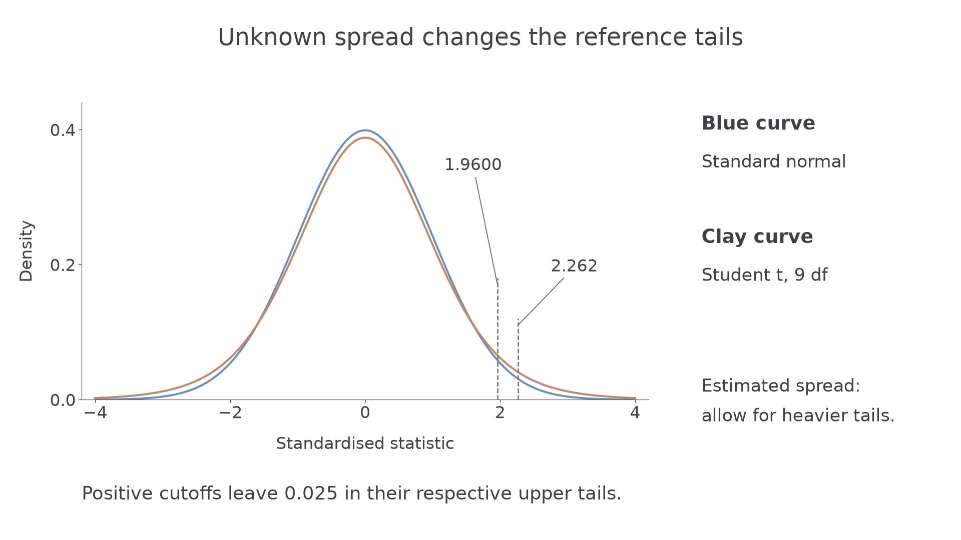
The assumption concerns the original population, not a claim that every small sample will look perfectly bell-shaped. Under this model, use the t procedure for unknown variance rather than silently replacing it with a z calculation.
Key idea
Estimate spread with the unbiased , use its square root in the standard error, and use degrees of freedom for the t reference distribution.
Identify what is known before selecting a procedure.
Test the mean with a tail chosen from the claim
Under , calculate . A positive alternative uses the upper tail; a negative alternative uses the lower tail. For a two-sided alternative, allocate half the significance level to each tail.
These hypothesis and tail-selection rules are applications of the supplied sampling distribution, rather than separately printed booklet formulas. Choose the alternative before seeing the observed sign.
Worked example 1: a positive one-tailed test
Question. Ten independent component lengths come from a normal population with unknown variance. The measurements in millimetres give
Test at whether the population mean length exceeds .
Plan. Find the unbiased spread, standardise the mean difference and compare with the upper point of .
Why this step? The variance is unknown, so estimating its square root in the denominator requires a t cutoff, not a normal cutoff.
Answer. Reject . There is sufficient evidence at that the population mean component length exceeds .
Check. The statistic is positive, agreeing with the direction of the claimed increase.
Worked example 2 changes only the pre-specified question to whether the mean differs in either direction.
Continue this lesson.
You’re previewing NovaLearn without an account. Create a free account to read the rest.
Create free account