FS2 4.1 - Linear combinations of normal variables
Independent normal variables remain normal when combined with fixed coefficients. You will find the mean and variance of a combination, translate comparisons into normal probabilities, and distinguish independent observations from repeated or shared readings.
Keep the signs in the mean and square them in the variance
Four independent readings and four times one reading have the same mean. Why can their variances differ by a factor of ? If each reading has distribution , the two totals both have mean , but their variances are and . The expression “four readings” needs a careful model.
You already know
From A-level Mathematics, records the mean and variance, not the standard deviation. For a normal variable, is standard normal; use the positive standard deviation when finding probabilities.
A coefficient can represent a change of scale, a subtraction or an average. A fixed added constant shifts every outcome by the same amount, so it changes the mean without adding spread.
Linear combination
A linear combination uses fixed coefficients, for example . Independence means the information from one variable does not change the distribution of the other. Separate normal distributions alone do not establish independence.
Means combine with their signed coefficients. For independent variables, variances combine with squared coefficients: a negative coefficient changes a deviation's sign before it is squared, so variance contributions still add.
The formula booklet supplies the independent variance algebra . The following full normal-distribution result also specifies the distribution's shape.
Independent normal combinations
If and independently, then for fixed real , and ,
provided the resulting variance is positive. A difference uses a negative coefficient; the variance contributions still add. You may use the normality result without proving it.
Not in the formula booklet: learn it.
The same rule extends to any finite collection of independent normal variables. Write each distinct independent variable once, then sum its coefficient times its mean and its squared coefficient times its variance.
Means still combine linearly without independence, but the simple variance addition needs independence. Readings sharing a calibration error, or expressions sharing the same observation, cannot automatically be treated as independent. If all random terms cancel, the result is a constant, rather than a normal variable with positive spread.
Key idea
Name the random quantity and check independence first. Signed coefficients determine its mean; squared coefficients determine its independent variance contributions.
Here is a diagnostic about the conditions, rather than the arithmetic.
Turn a comparison into one normal variable
Move every random term to one side of the inequality. The remaining fixed threshold tells you which tail or interval to use.
In the next pair, and are independent. The second parameters are variances, so their standard deviations are and .
Worked example 1: more than twice another reading
Question. Find the distribution of , and hence calculate .
Plan. Find the mean and variance of , then rewrite the event as and standardise.
Why use , rather than , for the variance? Subtraction affects the sign of 's contribution, but its deviations are multiplied by and then squared.
Answer. , and the probability is to three significant figures.
Check. The threshold is one standard deviation above the mean, so the upper-tail probability is below .
Worked example 2 changes only the coefficient of the same reading , from to .
Worked example 2: a different comparison coefficient
Question. Find the distribution of , and hence calculate .
Plan. Recalculate both parameters with coefficient , keeping the same threshold .
Why recalculate the mean as well as the variance? The coefficient changes the typical value of the combination and its spread; neither parameter stays fixed.
Answer. , and the probability is to three significant figures.
Check. The threshold is about standard deviations above the new mean, giving a smaller upper tail than in Worked example 1.
A condition such as becomes , so it uses two normal CDF values. A non-zero mean must still be subtracted at both endpoints.
Watch out
Wrong: standardise using the variance, such as . Right: divide by . Also square any standard deviations supplied in a context before forming the combined variance.
Pearson rewards the model, its parameters and the correctly translated event, so show them before the calculator output.
Exam tip
Write the combination's normal distribution and event explicitly. Keep unrounded parameters through the calculation, quote calculator probabilities with enough accuracy, then give the requested final rounding.
Change only that coefficient again.
A sum of observations is different from scaling one observation
Write subscripts when they mean different readings. has four independent sources of variation; has one source multiplied by .
[DIAGRAM: asset_name: Equal-mean normal totals with different dependence; asset_slug: 9fm0-fs2-127-sum-versus-scale; caption: Four independent readings have less spread than four times a single reading; description: A single coordinate plot compares two normal density curves centred at forty. The blue narrower density represents the sum of four independent observations each normal with mean ten and variance four, giving a normal total with mean forty and variance sixteen, standard deviation four. The clay wider density represents four times one observation, giving mean forty and variance sixty-four, standard deviation eight. Grey solid and dashed curve outlines distinguish the models, a vertical grey guide marks the common mean, and a clear legend explains both accents.]
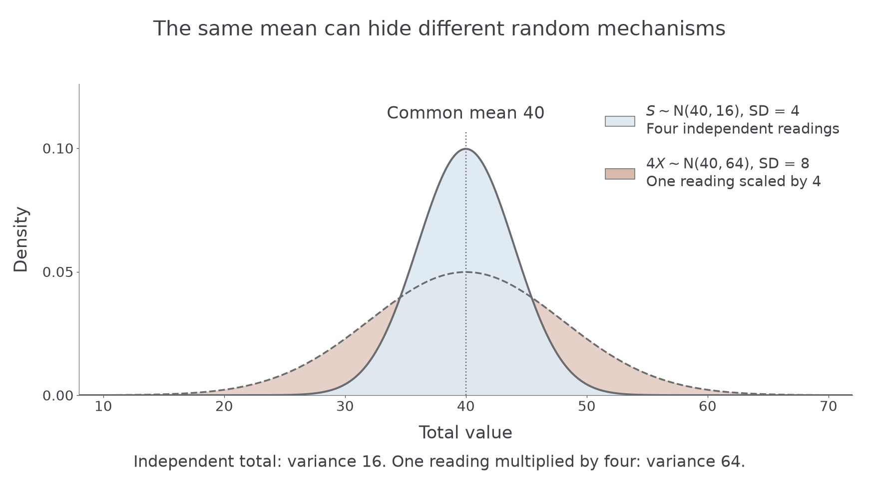
Independent normal totals and a scaled reading
For independent , each with distribution , let . Then
By contrast, scaling one reading gives
These distributions follow from the independent-combination and scaling rules; they are not printed separately.
Not in the formula booklet: learn it.
For the average , scaling the total gives mean and variance . The same average is commonly written .
Continue this lesson.
You’re previewing NovaLearn without an account. Create a free account to read the rest.
Create free account