CP 9.3 - Modelling with differential equations

You already know

An integrating factor solves $S'+P(t)S=Q(t)$; an initial amount selects the constant. Amount per unit volume is concentration, so multiplying concentration by volume flow rate gives amount per unit time.

Conservation in a mixing model

For tank volume $V(t)$, inflow rate $q_{\mathrm{in}}$, incoming concentration $c_{\mathrm{in}}(t)$, and outflow rate $q_{\mathrm{out}}$,

Assume uniform mixing and no other gain or loss of the substance. Equal volume flow rates make $V$ constant. Not in the formula booklet: learn it.

Worked example 1: constant incoming concentration

Question. A well-mixed tank contains $100\,\mathrm{L}$ of clean water. Solution enters at $2\,\mathrm{L\,min^{-1}}$, with concentration $3\,\mathrm{g\,L^{-1}}$; mixture leaves at the same volume rate. Form and solve a model for the mass $S$ grams after $t$ minutes, and find its limiting value.

Plan. Use constant volume, subtract the outgoing mass rate, then solve with $S(0)=0$.

Why this step? The leaving concentration is $S/100$, rather than the incoming value $3$: the tank starts clean and takes time to approach the inlet concentration.

Answer. $S=300(1-\mathrm{e}^{-t/50})\,\mathrm{g}$, with limiting mass $300\,\mathrm{g}$.

Check. $S(0)=0$, and $S'=6\mathrm{e}^{-t/50}=6-S/50$. At the limit, the tank concentration is $300/100=3\,\mathrm{g\,L^{-1}}$, equal to the incoming concentration.

Worked example 2: a falling input and a delayed peak

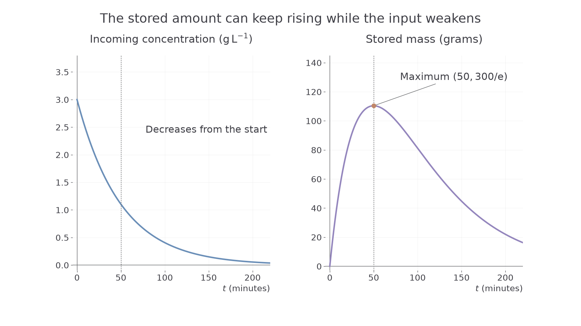
Question. The tank and flow rates are as in Worked example 1, but incoming concentration is $3\mathrm{e}^{-t/50}\,\mathrm{g\,L^{-1}}$. Find $S(t)$ and the time and value of its maximum.

Plan. Replace the incoming mass rate by $6\mathrm{e}^{-t/50}$, solve with the same factor and initial amount, then differentiate.

The derivative is positive for $0\le t<50$ and negative for $t>50$.

Why this step? The maximum occurs when incoming and outgoing mass rates balance, not when the incoming concentration itself is greatest.

Answer. $S=6t\mathrm{e}^{-t/50}\,\mathrm{g}$, with maximum $\frac{300}{\mathrm{e}}\,\mathrm{g}$, approximately $110\,\mathrm{g}$, at $t=50\,\mathrm{min}$.

Check. At $t=50$, both mass rates equal $6/\mathrm{e}\,\mathrm{g\,min^{-1}}$. Also $S\to0$ as $t\to\infty$, consistent with the fading input and continued flushing.

Watch out

Wrong: outflow mass rate $=S/100$. That is a concentration in $\mathrm{g\,L^{-1}}$. Right: multiply by the volume flow rate, giving $2S/100=S/50\,\mathrm{g\,min^{-1}}$.

You already know

In one-dimensional motion, $v=\frac{\mathrm{d}x}{\mathrm{d}t}$, $a=\frac{\mathrm{d}v}{\mathrm{d}t}$, and resultant force equals $ma$. Choose a positive direction and use signed forces. Integrating velocity gives displacement; its constant is set by the initial position.

Worked example 3: accelerating towards a limiting velocity

Question. A particle of mass $2\,\mathrm{kg}$ moves horizontally in the positive direction. A constant driving force is $8\,\mathrm{N}$; the opposing resistance has magnitude $v$ newtons when its speed is $v\,\mathrm{m\,s^{-1}}$. Initially $v=2$ and $x=0$. Find $v(t)$, $x(t)$ and the limiting velocity, using SI units.

Plan. Form the signed force balance, solve the linear velocity equation, then integrate velocity with the initial position.

Why this step? Resistance opposes the chosen positive motion, so it enters with a minus sign. A plus sign would predict ever-increasing acceleration instead of a balance.

Answer. $v=8-6\mathrm{e}^{-t/2}\,\mathrm{m\,s^{-1}}$, $x=8t-12(1-\mathrm{e}^{-t/2})\,\mathrm{m}$. The limiting velocity is $8\,\mathrm{m\,s^{-1}}$.

Check. At $t=0$, $v=2$ and $x=0$. Differentiating $x$ gives $v$; as $t\to\infty$, resistance tends to $8\,\mathrm{N}$, balancing the drive.