FP1 6.2 - Simpson's rule | Edexcel A-Level Further Mathematics

Estimate definite integrals by fitting parabolas through equally spaced ordinates (FP1 6.2). You will apply Simpson's rule with the correct weights, check that the grid is valid and reuse an estimate through algebraic relationships between integrals.

A parabola through three heights

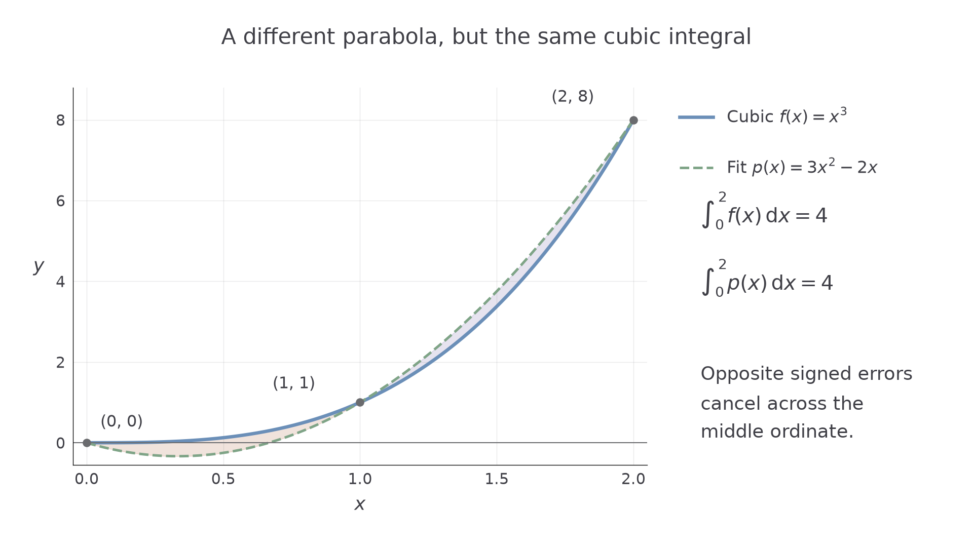
How can a method built from parabolas integrate a cubic exactly? Simpson's rule replaces each pair of intervals by the integral of a fitted quadratic. For a cubic, the two sides' errors cancel.

Begin with three heights $y_0,y_1,y_2$ , at equally spaced points $x_0,x_0+h,x_0+2h$ . The quadratic through them gives a better local description of curvature than a pair of straight-line edges.

You already know

A definite integral is signed accumulation; it can be negative. Constant multiples and sums can be taken through an integral, and a constant $c$ contributes $c(b-a)$ over $[a,b]$ . These are the assumed A-level Mathematics integration ideas; the new method concerns how to estimate an integral from ordinates.

For a short derivation, measure position from the middle point using $t=(x-x_1)/h$ . The fitted quadratic is

p(t)=y_1+\frac{y_2-y_0}{2}t+\frac{y_0-2y_1+y_2}{2}t^2

It takes the three given values at $t=-1,0,1$ . Integrating between $-1$ and $1$ , the odd term vanishes and $\mathrm dx=h\,\mathrm dt$ , giving

h\left[2y_1+\frac{y_0-2y_1+y_2}{3}\right] =\frac h3(y_0+4y_1+y_2)

This fitted-quadratic derivation is not supplied in the booklet.

Simpson's rule for two intervals

With equal interval width $h>0$ , and $y_j=f(x_0+jh)$ ,

\int_{x_0}^{x_0+2h}f(x)\,\mathrm dx \approx\frac h3(y_0+4y_1+y_2)

The three weights are $1,4,1$ . The rule integrates every polynomial of degree at most three exactly when the heights are exact; for general functions it is an approximation.

Not in the formula booklet: learn it.

The factor uses one interval's width $h$ , rather than the full width $2h$ .

Worked example 1: a quadratic panel

Question. Use Simpson's rule with two intervals to estimate $\int_0^2x^2\,\mathrm dx$ .

Plan. Use $h=1$ , find the three ordinates and apply weights $1,4,1$ .

\begin{aligned} h&=\frac{2-0}{2}=1 && \text{two equal intervals}\\ (y_0,y_1,y_2)&=(0,1,4) && \text{heights at }0,1,2\\ S&=\frac13[0+4(1)+4]=\frac83 && \text{weighted sum} \end{aligned}

Why this step? Integrating the fitted quadratic gives weights $1,4,1$ , with width factor $h/3$ ; keep both parts of that pattern intact.

Answer. The estimate is $8/3$ , and is exact for this quadratic.

Check. $[x^3/3]_0^2=8/3$ , agreeing with Simpson's value.

Change only the exponent of the integrand from $2$ to $3$ , retaining the same interval and grid.

Worked example 2: a cubic is exact too

Question. Use the same rule to estimate $\int_0^2x^3\,\mathrm dx$ .

Plan. Keep $h=1$ , update the three heights and compare with the exact integral.

\begin{aligned} (y_0,y_1,y_2)&=(0,1,8) && \text{cubic heights}\\ S&=\frac13[0+4(1)+8]=4 && \text{same weights}\\ \int_0^2x^3\,\mathrm dx&=\left[\frac{x^4}{4}\right]_0^2=4 && \text{exact comparison} \end{aligned}

Why this step? The fitted quadratic need not equal the original curve between the ordinates for their signed integrals to agree.

Answer. Simpson's estimate is exactly $4$ .

Check. The fitted quadratic is $p(x)=3x^2-2x$ , which also has integral $4$ . The difference $x^3-p(x)=x(x-1)(x-2)$ has opposite, cancelling contributions either side of $x=1$ .

The cubic's error relative to its fitted quadratic is odd about the panel's centre. Its integral therefore cancels over the symmetric panel. This explains the opening surprise; fitting a quadratic does not limit exact integration to quadratic functions.

[DIAGRAM: asset_name: A cubic and its Simpson quadratic; asset_slug: 9fm0-fp1-simpson-cubic; caption: The two signed errors cancel although the fitted parabola differs from the cubic; description: A Cartesian graph on x from 0 to 2 shows the cubic x cubed and the fitted quadratic 3x squared minus 2x. Their shared points (0,0), (1,1) and (2,8) are marked. Opposite shaded regions between the curves distinguish the error on the two halves. A separate legend and side panel state that both integrals are 4 and that the error changes sign about the middle ordinate.]
The two signed errors cancel although the fitted parabola differs from the cubic

Watch out

Exactness for a cubic does not make the rule exact for every smooth function. Also, Simpson's rule estimates a signed integral; geometric area below an axis needs the same sign care as exact integration.

Change only the integrand's exponent once more.

More panels and the alternating weights

For a longer table, combine the two-interval panels. Their shared endpoints are counted twice, producing the alternating interior weights.

The interval count $n$ must be even so that every interval belongs to a complete pair. That means an odd number $n+1$ of ordinates, including the two endpoints.

Composite Simpson's rule

For an even positive number $n$ of equal intervals, $h=(b-a)/n$ , $x_j=a+jh$ , $y_j=f(x_j)$ ,

\int_a^bf(x)\,\mathrm dx \approx\frac h3\left[ y_0+y_n +4(y_1+y_3+\cdots+y_{n-1}) +2(y_2+y_4+\cdots+y_{n-2}) \right]

The interior weight pattern is $4,2,4,2,\ldots,4$ . The endpoint weights are $1$ . The groups use ordinate indices, regardless of the numerical values of the $x$ -coordinates.

Not in the formula booklet: learn it.

Adding adjacent panels makes the pattern visible: the first panel contributes $y_0+4y_1+y_2$ , the next contributes $y_2+4y_3+y_4$ , and the shared $y_2$ therefore has total weight $2$ . The final endpoint belongs to only one panel.

Worked example 3: four intervals from a table

Question. Use all the tabulated values to estimate $\int_0^2\mathrm e^{-x^2}\,\mathrm dx$ , giving the answer to four decimal places.

$x$	$0$	$0.5$	$1$	$1.5$	$2$
$y=\mathrm e^{-x^2}$	$1.0000$	$0.7788$	$0.3679$	$0.1054$	$0.0183$

Plan. Count four intervals, use $h=0.5$ , and group endpoints, odd-indexed and even-indexed interior ordinates.

\begin{aligned} S&=\frac{0.5}{3}\left[ 1+0.0183+4(0.7788+0.1054)+2(0.3679) \right] && \text{all five ordinates}\\ &=\frac{5.2909}{6}=0.8818166\ldots && \text{evaluate before rounding} \end{aligned}

Why this step? Five heights make four intervals, so dividing the range by $5$ would give the wrong width.

Answer. The estimate is $0.8818$ to four decimal places.

Check. The positive decreasing integrand starts at $1$ and ends near $0.0183$ , so an integral between $0$ and $2$ is plausible. The weights are $1,4,2,4,1$ .

Continue this lesson.

You’re previewing NovaLearn without an account. Create a free account to read the rest.

Create free account

Last Accessed

Core Pure Mathematics

Further Pure Mathematics 1

Further Pure Mathematics 2

Further Statistics 1

Further Statistics 2

Further Mechanics 1

Further Mechanics 2

Decision Mathematics 1

Decision Mathematics 2

FP1 6.2 - Simpson's rule

A parabola through three heights

More panels and the alternating weights

Continue this lesson.

Learn faster with Nova