D1 5.4 - Two-stage Simplex and big-M methods | Edexcel A-Level Further Mathematics

Lower-bound and equality constraints may need temporary artificial variables before a feasible basis is available. You will use two-stage Simplex and big-M for maximisation and minimisation, remove artificial variables correctly and interpret parameterised final tableaux (D1 5.4).

A feasible basis is a starting point, not the optimum

For $x+y\ge4$ , $x+2y\le6$ , $x,y\ge0$ , a first stage finds $(x,y)=(4,0)$ with every artificial variable zero. Has it already optimised $3x+2y$ ?

It has found a genuine feasible plan, but feasibility and optimisation answer different questions. This same plan will turn out to be neither the maximum nor the minimum of that expression.

You already know

Subtract surplus from a $\ge$ row and add an artificial variable if an initial basic column is needed; an equality may need an artificial variable without surplus. Make right-hand sides non-negative first. Original feasibility requires all artificials to vanish. Ordinary Simplex uses a canonical feasible basis and exact row operations.

For the opening constraints, write

x+y-s_1+a_1=4,\qquad x+2y+s_2=6

Here $s_1$ is surplus, $s_2$ slack, and $a_1$ artificial. The computational starting basis is $a_1=4,s_2=6$ , with $x=y=s_1=0$ . It is not an original feasible plan.

First-stage objective

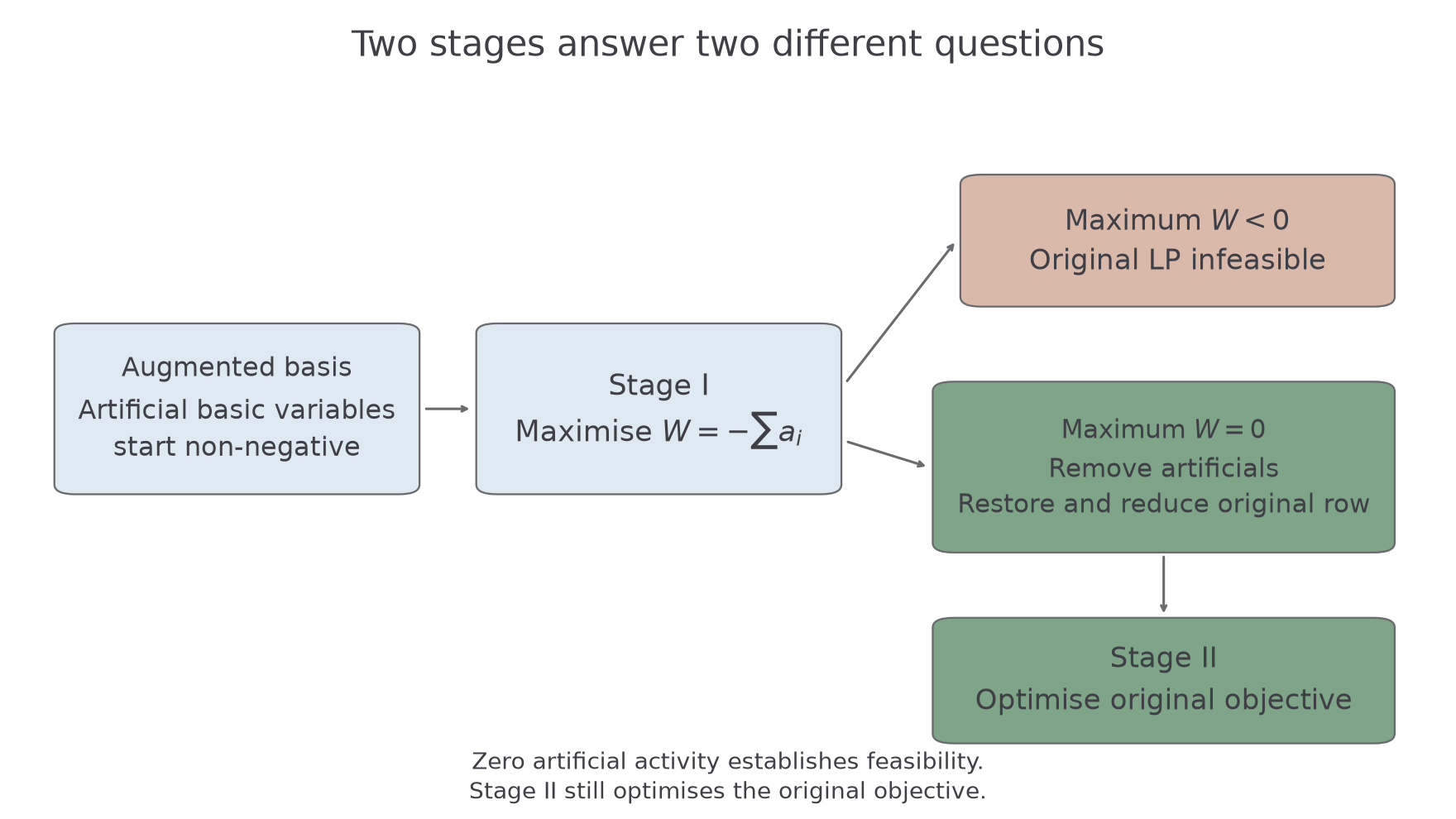
In the two-stage convention used here, maximise $W=-\sum_i a_i$ . Since each artificial variable is non-negative, $W\le0$ . If its maximum is $0$ , every artificial variable is zero and an original feasible basis can be obtained. If its maximum is negative, the original constraints are infeasible.

For example, $x\ge3$ , $x\le1$ , $x\ge0$ , gives $x-s+a=3$ . Since $x\le1$ and $s\ge0$ , $a=3-x+s\ge2$ . Thus the best $W=-a$ is $-2$ , attained at $x=1,s=0$ . No later optimisation can fix the incompatible original bounds.

An equality uses the same principle: $x+y=4$ may start as $x+y+a=4$ . It has no surplus term, and reaching $a=0$ restores the exact equality.

[DIAGRAM: asset_name: Two-stage Simplex separates feasibility from optimisation; asset_slug: 9fm0-d1-179-two-stage-flow; caption: A zero first-stage optimum permits the original objective to be restored; description: A left-to-right flow begins with adding artificial basic variables and then maximising W equal to minus the sum of artificial variables. A branch with maximum W below zero leads to original problem infeasible. A branch with maximum W zero leads to removing artificials and restoring the original objective, then to stage two optimising that objective. All arrows are full-opacity grey and the stage-two route is sage.]
A zero first-stage optimum permits the original objective to be restored

Key idea

Stage I asks whether the constraints can be satisfied without artificial help. Stage II optimises the original objective from a genuine feasible basis. A zero value of $W$ does not certify an original optimum.

Read the auxiliary objective as a feasibility certificate.

Find feasibility first, then restore the original objective

Use ordinary maximisation pivots on the auxiliary objective, then rebuild a canonical row for the original objective.

Two-stage Simplex

Form non-negative slack, surplus and artificial variables with an initial feasible augmented basis.
Set $W=-\sum a_i$ . Eliminate basic artificial variables from its row before pivoting.
Maximise $W$ by Simplex. A negative optimum means the original problem is infeasible; an optimum zero permits Stage II.
Remove artificials from the basis and delete their columns and the $W$ row. Restore the original objective, converting minimisation to maximisation if needed.
Eliminate every current basic variable from that objective row, then continue Simplex and interpret the original result.

Not in the formula booklet: learn it.

An artificial variable can remain basic at value zero when Stage I ends. Pivot it out using a non-zero non-artificial non-basic coefficient in its zero-Value row. This keeps right-hand sides feasible. If that row has no such coefficient, it is redundant after artificials are set to zero and can be removed. For example, $2x+a=0$ permits a pivot on $2$ to make $x=0$ basic; a row consisting only of $a=0$ is removed. Do not delete a non-redundant constraint merely because its artificial value is zero.

Worked example 1: a maximisation after feasibility

Question. Use two-stage Simplex to maximise $P=3x+2y$ , subject to $x+y\ge4$ , $x+2y\le6$ , $x,y\ge0$ .

Plan. First maximise $W=-a_1$ , then remove $a_1$ and restore a canonical row for $P$ .

The augmented constraints are those above. From $W+a_1=0$ , subtract the first constraint to eliminate basic $a_1$ :

W-x-y+s_1=-4

b.v.	$x$	$y$	$s_1$	$s_2$	$a_1$	Value
$a_1$	$1$	$1$	$-1$	$0$	$1$	$4$
$s_2$	$1$	$2$	$0$	$1$	$0$	$6$
$W$	$-1$	$-1$	$1$	$0$	$0$	$-4$

Choose $x$ from the tied entering columns. Ratios $4,6$ select row $1$ ; $a_1$ leaves. Use $R_2\leftarrow R_2-R_1$ , $R_W\leftarrow R_W+R_1$ :

b.v.	$x$	$y$	$s_1$	$s_2$	$a_1$	Value
$x$	$1$	$1$	$-1$	$0$	$1$	$4$
$s_2$	$0$	$1$	$1$	$1$	$-1$	$2$
$W$	$0$	$0$	$0$	$0$	$1$	$0$

Stage I has optimum $W=0$ , with non-basic $a_1=0$ . Delete its column and the $W$ row. Restore $P-3x-2y=0$ ; add $3R_1$ to eliminate basic $x$ :

b.v.	$x$	$y$	$s_1$	$s_2$	Value
$x$	$1$	$1$	$-1$	$0$	$4$
$s_2$	$0$	$1$	$1$	$1$	$2$
$P$	$0$	$1$	$-3$	$0$	$12$

Enter surplus $s_1$ : only row $2$ has a positive entry, giving ratio $2$ . Use $R_1\leftarrow R_1+R_2$ , $R_P\leftarrow R_P+3R_2$ , and relabel row $2$ :

b.v.	$x$	$y$	$s_1$	$s_2$	Value
$x$	$1$	$2$	$0$	$1$	$6$
$s_1$	$0$	$1$	$1$	$1$	$2$
$P$	$0$	$4$	$0$	$3$	$18$

Why this step? Restoring the raw objective is insufficient: the current basic $x$ must have zero coefficient in its row. A surplus variable can enter just like any other non-basic variable.

Answer. Set $y=s_2=0$ : $x=6$ , maximum $P=18$ .

Check. The first constraint has surplus $2$ , the second is tight, and $P=18-4y-3s_2\le18$ . The Stage I point had objective $12$ , so finding feasibility did not finish maximisation.

Worked example 2 changes only the required direction of optimisation of $3x+2y$ , from maximum to minimum. Stage I is unchanged; Stage II must use a different objective.

Worked example 2: the same feasible start, a minimum instead

Question. Use two-stage Simplex to minimise $C=3x+2y$ under the same constraints.

Plan. Repeat the auxiliary feasibility stage, then maximise $P=-C$ .

The first-stage initial tableau is

b.v.	$x$	$y$	$s_1$	$s_2$	$a_1$	Value
$a_1$	$1$	$1$	$-1$	$0$	$1$	$4$
$s_2$	$1$	$2$	$0$	$1$	$0$	$6$
$W$	$-1$	$-1$	$1$	$0$	$0$	$-4$

Enter $x$ , using ratios $4,6$ , and apply $R_2\leftarrow R_2-R_1$ , $R_W\leftarrow R_W+R_1$ :

b.v.	$x$	$y$	$s_1$	$s_2$	$a_1$	Value
$x$	$1$	$1$	$-1$	$0$	$1$	$4$
$s_2$	$0$	$1$	$1$	$1$	$-1$	$2$
$W$	$0$	$0$	$0$	$0$	$1$	$0$

Remove the non-basic artificial column and $W$ . The original converted row is $P+3x+2y=0$ . Apply $R_P\leftarrow R_P-3R_1$ :

b.v.	$x$	$y$	$s_1$	$s_2$	Value
$x$	$1$	$1$	$-1$	$0$	$4$
$s_2$	$0$	$1$	$1$	$1$	$2$
$P$	$0$	$-1$	$3$	$0$	$-12$

Enter $y$ . Ratios $4,2$ select row $2$ . Use $R_1\leftarrow R_1-R_2$ , $R_P\leftarrow R_P+R_2$ :

b.v.	$x$	$y$	$s_1$	$s_2$	Value
$x$	$1$	$0$	$-2$	$-1$	$2$
$y$	$0$	$1$	$1$	$1$	$2$
$P$	$0$	$0$	$4$	$1$	$-10$

Why this step? The auxiliary objective does not depend on whether the original question asks for a maximum or minimum. The restored objective does, so its signs must be changed before Stage II.

Answer. $x=y=2$ , maximum $P=-10$ , hence minimum $C=10$ .

Check. Both original constraints hold with equality. Since $P=-10-4s_1-s_2\le-10$ , the original cost satisfies $C\ge10$ .

An optimum in a feasible Stage II tableau follows the ordinary Simplex tests, including the checks for unbounded directions or alternative optimal solutions. The extra work was obtaining a genuine basis and the correct restored row.

Watch out

Wrong: stop as soon as $W=0$ , or replace the auxiliary row by an unreduced original row containing basic-variable coefficients. Right: clean up the artificial basis, restore the original objective and eliminate every current basic variable before continuing.

Change only the original cost's $x$ coefficient in the next check.

Continue this lesson.

You’re previewing NovaLearn without an account. Create a free account to read the rest.

Create free account

Last Accessed

Core Pure Mathematics

Further Pure Mathematics 1

Further Pure Mathematics 2

Further Statistics 1

Further Statistics 2

Further Mechanics 1

Further Mechanics 2

Decision Mathematics 1

Decision Mathematics 2

D1 5.4 - Two-stage Simplex and big-M methods

A feasible basis is a starting point, not the optimum

Find feasibility first, then restore the original objective

Continue this lesson.

Learn faster with Nova