FS2 2.4 - The continuous uniform distribution | Edexcel A-Level Further Mathematics

A uniform density gives equal probabilities to equal-length intervals within its support. You will derive its CDF, mean and variance, use interval lengths for probabilities and conditional probabilities, and calculate expectations of quantities that depend on a uniform random measurement.

A rectangle turns probability into a length ratio

A random height has mean $3$ . Why can a triangle built from it have mean area $\frac{14}{3}$ , rather than the area $\frac92$ obtained by using height $3$ ? Equal density does not make nonlinear averaging disappear. First build the simplest continuous model; then you will use it on that triangle.

You already know

A density has total area $1$ . Its CDF accumulates area from the left, interval probabilities are CDF differences, and $\mathrm E(g(X))=\int g(x)f(x)\,\mathrm{d}x$ averages the transformed value.

If every equal-length interval inside $[a,b]$ has the same probability, the density must have one constant height. A rectangle of width $b-a$ needs height $1/(b-a)$ to have area $1$ .

Continuous uniform distribution

Write $X\sim\mathrm U[a,b]$ , where $a<b$ , when $X$ has constant density on $[a,b]$ and zero density elsewhere. It is also called a rectangular distribution. Equal-length subintervals of the support have equal probabilities; individual point probabilities are still zero.

The interval needs positive width. When $a=b$ , this density formula is undefined; a fixed value is a different kind of model.

Uniform density

For $X\sim\mathrm U[a,b]$ , with $a<b$ ,

f(x)= \begin{cases} \frac1{b-a} & a\le x\le b\\ 0 & \text{otherwise} \end{cases}

In the formula booklet.

The CDF is obtained by integrating this rectangle. Below $a$ there is no area; above $b$ all the area has accumulated. Between the endpoints,

F(x)=\int_a^x\frac1{b-a}\,\mathrm{d}t =\frac{x-a}{b-a}

This is the required derivation, rather than a new formula to quote without explanation.

Uniform CDF

F(x)= \begin{cases} 0 & x<a\\ \frac{x-a}{b-a} & a\le x\le b\\ 1 & x>b \end{cases}

The middle branch is the accumulated width divided by the total width.

Not in the formula booklet: learn it.

For $a\le u<v\le b$ , its difference gives $\mathrm P(u<X<v)=\frac{v-u}{b-a}$ , a derived length ratio rather than a separately printed booklet formula. If a requested interval extends beyond the support, use only its overlap with $[a,b]$ .

[DIAGRAM: asset_name: Uniform density rectangle and linear cumulative distribution; asset_slug: 9fm0-fs2-123-uniform-cdf; caption: The shaded interval probability is its width divided by the whole support width; description: Two coordinate panels show X uniform on minus two to six. The density panel has a constant rectangle of height one eighth and total area one, with the interval one to four shaded in sage and labelled area three eighths. The CDF panel is zero to the left of minus two, rises linearly from minus two comma zero to six comma one, and stays one afterwards. Guides show F of one equals three eighths and F of four equals three quarters. Axes, support endpoints and all labels are clear.]
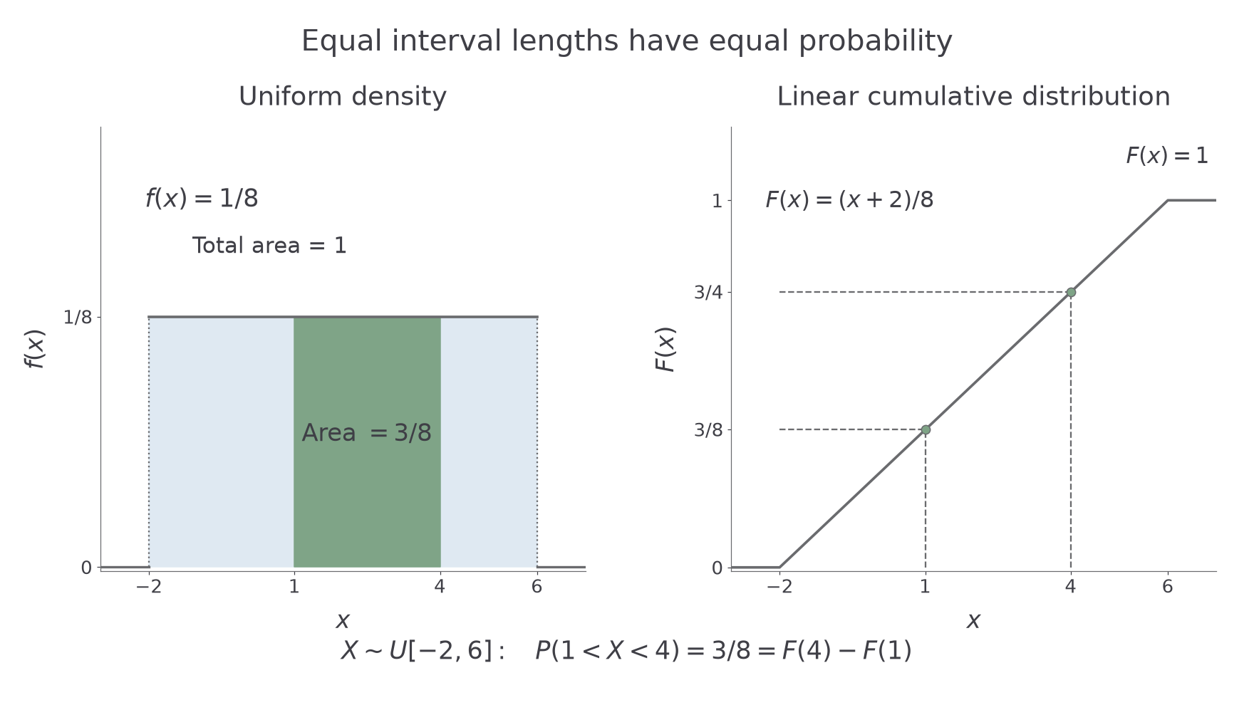
The shaded interval probability is its width divided by the whole support width

Worked example 1: a support crossing zero

Question. $X\sim\mathrm U[-2,6]$ . Find its CDF and $\mathrm P(1<X<4)$ .

Plan. Use total width $8$ , integrate the constant density from $-2$ , and compare interval lengths.

\begin{aligned} f(x)&=\frac18 && -2\le x\le6\\ F(x)&=\int_{-2}^{x}\frac18\,\mathrm{d}t =\frac{x+2}{8} && -2\le x\le6\\ \mathrm P(1<X<4)&=\frac{4-1}{6-(-2)} =\frac38 && \text{desired width over total width} \end{aligned}

Why use $x+2$ ? The accumulated interval starts at $-2$ , so its width is $x-(-2)$ , rather than $x$ .

Answer.

F(x)= \begin{cases} 0 & x<-2\\ \frac{x+2}{8} & -2\le x\le6\\ 1 & x>6 \end{cases} \qquad \mathrm P(1<X<4)=\frac38

Check. $F(-2)=0$ , $F(6)=1$ , and $F(4)-F(1)=\frac68-\frac38=\frac38$ .

Worked example 2 changes only the upper endpoint, stretching the same total probability over a longer interval.

Worked example 2: a wider support lowers the density

Question. Now $X\sim\mathrm U[-2,10]$ . Find its CDF and $\mathrm P(1<X<4)$ .

Plan. Replace the total width by $12$ , keeping the same requested interval.

\begin{aligned} f(x)&=\frac1{12} && -2\le x\le10\\ F(x)&=\int_{-2}^x\frac1{12}\,\mathrm{d}t =\frac{x+2}{12} && \text{new accumulated fraction}\\ \mathrm P(1<X<4)&=\frac3{12}=\frac14 && \text{same width, lower height} \end{aligned}

Why does the probability fall? The interval $(1,4)$ now occupies a smaller fraction of the support.

Answer. The CDF is $0$ below $-2$ , $\frac{x+2}{12}$ on $[-2,10]$ , and $1$ above $10$ ; the probability is $\frac14$ .

Check. The rectangle area is $12\times\frac1{12}=1$ , and $F(4)-F(1)=\frac6{12}-\frac3{12}=\frac14$ .

A uniform model is appropriate only when constant density is credible over the stated interval. Knowing only the minimum and maximum does not establish uniformity.

Watch out

Wrong: divide by the upper endpoint $b$ . Right: divide by the width $b-a$ . For $[-2,6]$ , the width is $8$ , not $6$ .

Stretch that upper endpoint again.

Derive the mean and variance before using them

The centre of a rectangle suggests its mean. Integration confirms that intuition and gives the spread as well.

For $X\sim\mathrm U[a,b]$ , the expectation integral gives

\begin{aligned} \mathrm E(X)&=\frac1{b-a}\int_a^b x\,\mathrm{d}x =\frac{b^2-a^2}{2(b-a)} =\frac{a+b}{2} && \text{factor the difference of squares}\\ \mathrm E(X^2)&=\frac1{b-a}\int_a^b x^2\,\mathrm{d}x =\frac{b^3-a^3}{3(b-a)} =\frac{a^2+ab+b^2}{3} && \text{factor the difference of cubes}\\ \operatorname{Var}(X)&=\frac{a^2+ab+b^2}{3} -\left(\frac{a+b}{2}\right)^2 && \text{second moment minus squared mean}\\ &=\frac{4a^2+4ab+4b^2-3a^2-6ab-3b^2}{12} =\frac{(b-a)^2}{12} && \text{simplify} \end{aligned}

These derivations may be required, even though their final results are supplied.

Uniform mean and variance

For $X\sim\mathrm U[a,b]$ , with $a<b$ ,

\mathrm E(X)=\frac{a+b}{2}, \qquad \operatorname{Var}(X)=\frac{(b-a)^2}{12}

In the formula booklet.

The mean determines the midpoint; the variance determines the width. Moving the whole interval changes the mean but leaves the variance unchanged. Multiplying its width by a factor multiplies its variance by that factor squared.

Worked example 3: recover the two endpoints

Question. A uniform variable has mean $5$ and variance $3$ . Find its support $[a,b]$ .

Plan. Find the midpoint and positive width, then move half that width either side of the midpoint.

\begin{aligned} a+b&=10 && \text{twice the mean}\\ (b-a)^2&=12\times3=36 && \text{use the variance}\\ b-a&=6 && \text{width is positive}\\ a&=\frac{10-6}{2}=2,\qquad b=\frac{10+6}{2}=8 && \text{solve sum and difference} \end{aligned}

Why choose the positive root? By definition $a<b$ , so $b-a$ is a width, not a signed displacement.

Answer. The support is $[2,8]$ .

Check. Its midpoint is $5$ , and its variance is $\frac{6^2}{12}=3$ .

Worked example 4 changes only the variance. The midpoint stays at $5$ .

Worked example 4: four times the variance

Question. A uniform variable has mean $5$ and variance $12$ . Find its support.

Plan. Find the new positive width from the variance, keeping the same midpoint.

\begin{aligned} a+b&=10 && \text{unchanged mean}\\ b-a&=\sqrt{12\times12}=12 && \text{positive width}\\ a&=\frac{10-12}{2}=-1,\qquad b=\frac{10+12}{2}=11 && \text{solve for endpoints} \end{aligned}

Why does the width only double? Variance depends on width squared, so multiplying variance by $4$ multiplies width by $2$ .

Answer. The support is $[-1,11]$ .

Check. The midpoint is $\frac{-1+11}{2}=5$ , and $\frac{12^2}{12}=12$ .

The CDF also shows that the midpoint cuts the area in half. More generally, the cut leaving probability $p$ to the left is $a+p(b-a)$ , obtained by solving $(x-a)/(b-a)=p$ . This percentile expression is derived, rather than printed separately in the booklet. The flat density has no unique modal peak.

Watch out

Wrong: $\operatorname{Var}(X)=\frac{b-a}{12}$ . Right: square the width. Also distinguish variance from standard deviation when recovering the endpoints.

Continue this lesson.

You’re previewing NovaLearn without an account. Create a free account to read the rest.

Create free account

Last Accessed

Core Pure Mathematics

Further Pure Mathematics 1

Further Pure Mathematics 2

Further Statistics 1

Further Statistics 2

Further Mechanics 1

Further Mechanics 2

Decision Mathematics 1

Decision Mathematics 2

FS2 2.4 - The continuous uniform distribution

A rectangle turns probability into a length ratio

Derive the mean and variance before using them

Continue this lesson.

Learn faster with Nova