FS1 4.2 - Testing a geometric parameter | Edexcel A-Level Further Mathematics

A long wait for success can challenge a claimed success probability. You will test the population parameter of a geometric distribution, choose the correct tail, construct integer critical regions and check their actual significance levels (FS1 4.2).

A longer wait points to a smaller probability

A spinner is supposed to land on red with probability $0.2$ . You spin independently until the first red, which arrives on spin $14$ . Is this enough evidence, at the $5\%$ level, that the probability of red is lower than claimed?

Here a large observation supports a small parameter. That reverses the relationship in a Poisson mean test: reducing a geometric success probability makes long waits more likely.

You already know

If $X\sim\operatorname{Geo}(p)$ , $X$ counts all trials up to and including the first success, so $X=1,2,\ldots$ . For $q=1-p$ , $\mathrm P(X\ge x)=q^{x-1}$ and $\mathrm P(X\le x)=1-q^x$ . The probability formula $p(1-p)^{x-1}$ is supplied in the booklet; these tail forms are derived, not printed.

Define $p$ as the population probability of red on each spin. For the opening claim, write $H_0:p=0.2$ , $H_1:p<0.2$ , and use $X\sim\operatorname{Geo}(0.2)$ under $H_0$ . The observation $x=14$ is a trial number, not an estimate to insert into the hypotheses.

Claim	Alternative	Evidence supporting it	One-sided tail under the null
Success has become less likely	$p<p_0$	A long wait	$\mathrm P(X\ge x)$
Success has become more likely	$p>p_0$	A short wait	$\mathrm P(X\le x)$
The probability has changed	$p\ne p_0$	Either extreme	Both tails

The trials must be independent with the same success probability. “Success” is simply the named event; it may be a fault, a six or a fault-free run. Repeated sampling without replacement or a player improving with practice can break the model. Do not change the stopping rule to a fixed number of trials: that creates a different experiment.

A useful warning comes from $p_0=0.02$ . Every individual geometric probability is at most $0.02$ , since $0.02(0.98)^{x-1}\le0.02$ . A supposed $5\%$ test that rejected whenever an individual outcome had probability below $0.05$ would reject on every possible result, even when $p=0.02$ ! Extremeness requires a tail, not just a small point probability.

Key idea

Choose the alternative from the claim, then choose the tail from the waiting-time meaning: small $p$ goes with large $X$ . A non-significant result gives insufficient evidence for the alternative; it does not establish that $p=p_0$ .

Keep the population parameter and the observed waiting time separate in this check.

Testing an observed first-success trial

Calculate the inclusive tail under $p_0$ , compare it with the stated level, and give a contextual conclusion about the population probability.

One-sided geometric tests

For $X\sim\operatorname{Geo}(p_0)$ under $H_0$ , where $0<p_0<1$ , an observed trial $x$ gives

\begin{array}{c|c} H_1:p<p_0&\mathrm P(X\ge x)=(1-p_0)^{x-1}\\ H_1:p>p_0&\mathrm P(X\le x)=1-(1-p_0)^x \end{array}

Reject $H_0$ if the relevant probability is at most the stated significance level $\alpha$ .

Not in the formula booklet: learn it.

For a long-wait test, reaching trial $x$ requires failures on the first $x-1$ trials. It does not require success exactly at $x$ ; later successes count as at least as extreme too.

[DIAGRAM: asset_name: The geometric test tail includes later successes; asset_slug: 9fm0-fs109-geometric-test-tail; caption: First success on trial fourteen is tested using thirteen initial failures and every later possible success; description: A timeline shows thirteen pale blue F cells followed by a sage S cell on trial fourteen, labelled as the observed outcome. A bracket under the first thirteen cells identifies the failures needed for the event X at least fourteen. The upper-tail probability is 0.8 to the power thirteen, approximately 0.05498. Text states that the test tail also includes first successes on trials fifteen, sixteen and all later trials, and that multiplying by 0.2 would instead give the point probability for exactly fourteen.]
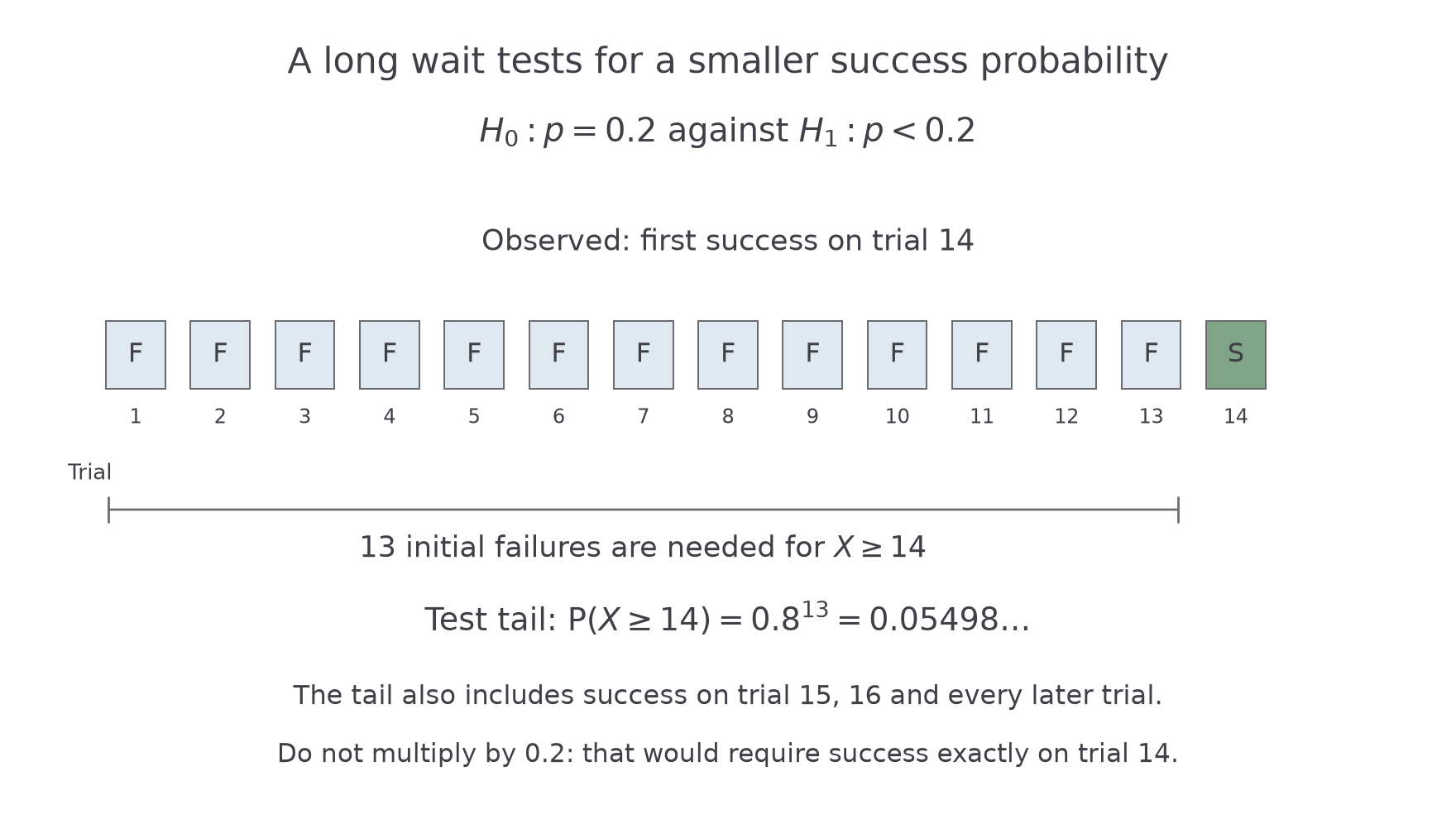
First success on trial fourteen is tested using thirteen initial failures and every later possible success

Worked example 1: fourteen trials are not quite enough

Question. A spinner has population probability $p$ of red on each independent spin. The first red occurs on spin $14$ . Test $H_0:p=0.2$ against $H_1:p<0.2$ at the $5\%$ level.

Plan. A long wait supports the alternative, so use the upper geometric tail under $p_0=0.2$ .

\begin{aligned} X&\sim\operatorname{Geo}(0.2)\text{ under }H_0 &&\text{trial of first red}\\ \mathrm P(X\ge14)&=(0.8)^{13} &&\text{thirteen initial failures}\\ &=0.0549755\ldots &&\text{evaluate the whole tail}\\ 0.0549755\ldots&>0.05 &&\text{not significant} \end{aligned}

Why this step? $\mathrm P(X=14)=0.2(0.8)^{13}$ would count only one stopping trial. It omits every longer wait, even though longer waits support a reduction still more strongly.

Answer. Do not reject $H_0$ . At the $5\%$ level there is insufficient evidence that the population probability of red is less than $0.2$ .

Check. The point probability is only $0.0109951\ldots$ , but the correct tail is larger. The decision must use $0.0549755\ldots$ , without rounding it prematurely to $0.05$ .

Worked example 2 changes only the observed first-red trial, from $14$ to $15$ . All test choices stay fixed.

Worked example 2: one extra failure changes the decision

Question. Carry out the same test if the first red occurs on spin $15$ .

Plan. Include all waits of at least $15$ under the same null model.

\begin{aligned} H_0&:p=0.2,\qquad H_1:p<0.2 &&\text{same hypotheses}\\ \mathrm P(X\ge15)&=(0.8)^{14} &&\text{fourteen initial failures}\\ &=0.0439804\ldots<0.05 &&\text{significant upper tail} \end{aligned}

Why this step? One extra required failure multiplies the preceding tail by $0.8$ , taking it below the $5\%$ boundary.

Answer. Reject $H_0$ . There is sufficient evidence, at the $5\%$ level, that the population probability of red is below $0.2$ .

Check. The adjacent tails straddle $0.05$ , so this test's critical region is $X\ge15$ . Its actual significance is $0.0439804\ldots$ , not exactly $0.05$ .

For the opposite alternative $p>p_0$ , the lower-tail probability starts at $\mathrm P(X\le1)=p_0$ . If $p_0=0.2$ , even an immediate success has lower-tail probability $0.2>0.05$ . No non-empty short-wait critical region is possible for a one-observation $5\%$ test of that increase. This is a limitation of the experiment, not an arithmetic error.

Continue this lesson.

You’re previewing NovaLearn without an account. Create a free account to read the rest.

Create free account

Last Accessed

Core Pure Mathematics

Further Pure Mathematics 1

Further Pure Mathematics 2

Further Statistics 1

Further Statistics 2

Further Mechanics 1

Further Mechanics 2

Decision Mathematics 1

Decision Mathematics 2

FS1 4.2 - Testing a geometric parameter

A longer wait points to a smaller probability

Testing an observed first-success trial

Continue this lesson.

Learn faster with Nova