FP2 3.1 - Eigenvalues and eigenvectors
Find the directions that a matrix stretches without turning away from their own line. Calculate eigenvalues and eigenvectors of two by two and three by three matrices, including zero, repeated and complex eigenvalues, and give normalised vectors when requested.
Directions that survive a transformation
Can a real matrix have no real direction that survives its action? A quarter-turn seems a promising candidate: every non-zero real vector turns through a right angle. Yet it will still have eigenvalues once we allow complex numbers. That small surprise connects the geometry you know to a much wider algebra.
You already know
Matrix multiplication gives the image of a column vector. An invariant point satisfies ; an invariant line need not consist of fixed points. A square matrix is singular exactly when its determinant is zero. Use the two by two determinant or cofactor expansion from Core Pure.
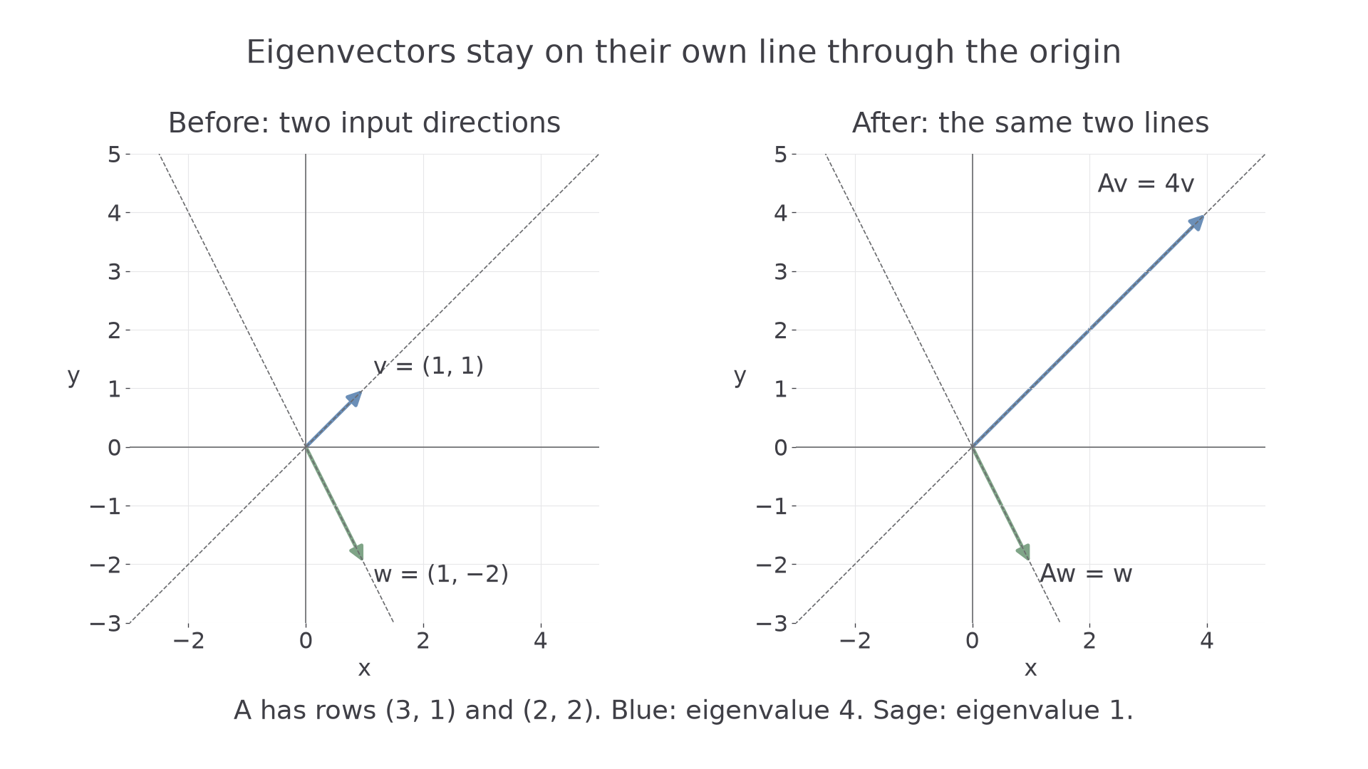
For , multiplying gives . Its length changes but its direction does not. Multiplying gives the same vector back. These are especially convenient directions for this particular matrix.
[DIAGRAM: asset_name: Two eigenvector directions under a matrix; asset_slug: 9fm0-fp294-eigendirections; caption: The blue direction is stretched by 4 while the sage direction is fixed; description: Equal-scale coordinate panels show vectors v=(1,1) and w=(1,-2) before transformation and their images (4,4) and (1,-2) under A with rows (3,1) and (2,2). Blue highlights the first direction and sage the second. Grey dashed complete lines distinguish directions from individual vectors. All labels are ink.]
Eigenvalue and eigenvector
For a square matrix , a non-zero vector is an eigenvector with eigenvalue when
For real vectors and real , the image remains on the same line through the origin: a negative eigenvalue reverses direction; eigenvalue fixes the vector; eigenvalue sends it to the origin.
The zero vector satisfies the equation for every , so allowing it would tell us nothing. A zero eigenvalue is perfectly valid; a zero eigenvector is not. Any non-zero scalar multiple of an eigenvector is another eigenvector for the same eigenvalue, because .
Key idea
An eigenvector is a non-zero input whose image is a scalar multiple of itself. Always keep its eigenvalue attached to it.
Neither the eigenvector definition nor the methods in this lesson are supplied in the formula booklet. The next check separates the two different roles of zero.
Find eigenvalues and eigenvectors in two dimensions
Rearrange the defining equation to . A non-zero solution exists only when the coefficient matrix is singular. Its determinant therefore gives the equation for . Subtract from diagonal entries only.
Characteristic equation
For an by matrix,
is the characteristic equation. For , it is
For each root, solve and choose a non-zero solution. The equivalent equation has the same roots.
Not in the formula booklet: learn it.
The determinant is the route to the eigenvalues, not the final eigenvectors. Those come from simultaneous linear equations.
Worked example 1: two distinct eigenvalues
Question. Find the eigenvalues and a corresponding eigenvector for each for .
Plan. Solve the characteristic equation, then substitute each eigenvalue into the vector equation.
For , the first row gives
Why this step? Each singular system has a free scale. Choosing a convenient non-zero value gives one representative, not a unique vector.
Answer. The eigenpairs are and , allowing non-zero multiples of either vector.
Check. The products are and , agreeing with both eigenvalues.
Change only the lower-left entry, from to . One eigenvalue becomes zero; retain it.
Worked example 2: a singular matrix still has eigenvectors
Question. Find the eigenvalues and corresponding eigenvectors of .
Plan. Use the same determinant and first-row equations, checking the second row afterwards.
Why this step? The matrix is singular, so some non-zero inputs must collapse to zero. They supply the eigenvectors for eigenvalue zero.
Answer. Eigenvalue has eigenvectors ; eigenvalue has eigenvectors , with in each case.
Check. and .
The equation must subtract the scalar times the identity, not the scalar from every entry.
Watch out
Wrong: replace by . Right: the off-diagonal entries stay and , because the identity has zeros there.
Change the lower-left entry once more, keeping the same method.
Work systematically with three coordinates
For three by three matrices, the characteristic equation is cubic. A zero entry can simplify its expansion. A supplied eigenvalue gives a known factor; substitute it into the polynomial before dividing. Once a root is known, use enough component equations to establish a vector and check all three rows.
Worked example 3: use a simple root of a cubic
Question. Find the eigenvalues and corresponding eigenvectors of .
Plan. Expand along the first row, factor out , then solve the component equations.
Thus . For , the outer rows give , and the middle row gives . For the other roots, the outer rows give , so .
Why this step? Dividing by would lose the root . Handle it before using that non-zero factor.
Answer. The eigenvalues are , with corresponding eigenvectors above.
Check. Their images are , and , respectively.
Change only the central entry from to . The factorisation strategy survives, but the other two eigenvalues change.
Worked example 4: change one entry and retain a zero eigenvalue
Question. Find the eigenvalues and corresponding eigenvectors of .
Plan. Repeat the first-row expansion and separate the root when solving for vectors.
Why this step? The outer rows determine the same relationships as before, but the changed middle row determines which eigenvalues make them consistent.
Answer. The eigenvalues are , with the corresponding vectors shown.
Check. Multiplication gives , and , in that order.
Any vector found from one equation must satisfy the remaining equations too. The determinant guarantees existence, not the correctness of your chosen components.
Watch out
Wrong: for , cancel and conclude . Right: substitute first; the middle equation gives . Dividing by zero would replace the correct direction by a wrong one.
One more change to the central entry introduces exact surds rather than new methods.
Continue this lesson.
You’re previewing NovaLearn without an account. Create a free account to read the rest.
Create free account