FS1 2.1 - The Poisson distribution
Random arrivals do not have to arrive in a regular pattern for their counts to have a useful model. You will decide when a Poisson distribution is reasonable, calculate point and cumulative probabilities and keep the endpoints of discrete probability events exact.
A model for random event counts
A small online shop receives an average of three orders in a ten-minute period. Under a Poisson model, is exactly three orders more likely than exactly two? The answer is surprising: those two counts have exactly the same probability. We will calculate it, rather than treating an average as a guaranteed outcome.
You already know
A discrete random variable has separate possible values, with probabilities adding to . Write for a point probability. The mean describes a long-run average; it need not be the count in any particular observation.
The Poisson distribution models the number of events in a specified interval. The interval might be ten minutes, a length of cable or an area of material. Define it before giving the parameter: “three per ten minutes” and “three per hour” are different models.
Poisson distribution
A count has a Poisson distribution with parameter , written , when
The parameter is the expected number of events in the chosen interval. Zero is a possible count, and there is no fixed upper count. A waiting time measured continuously is not a Poisson count.
To use this as an event-count model, look for three features:
- Events occur independently: one arrival does not trigger or prevent another.
- Events occur at a constant average rate throughout the interval being modelled.
- Events occur singly, rather than in inseparable batches; multiple events in a sufficiently short interval are negligible.
“Constant rate” does not mean the same number occurs every minute. It means that equal-length parts of the interval have the same expected count. “Random” alone is also insufficient: a randomly timed promotion might still generate clusters of orders.
For the shop, a steady quiet period could be plausible. A sale announcement could increase the order rate, while customers sharing a limited-stock link could make arrivals dependent. State the particular assumption affected, rather than merely saying that real life is unpredictable.
Key idea
Use a Poisson model for a count over a defined interval when independence, a constant rate and single-event arrivals are reasonable. Criticise the assumption in the context of the events.
The following check distinguishes a rate from a fixed count.
Point probabilities and the parameter
Use the Poisson probability formula for an exact count, keeping the parameter for the stated interval and the factorial for the requested integer.
Poisson point probability
For , with ,
Since , .
In the formula booklet.
A calculator's Poisson probability function evaluates this point probability. Its cumulative function answers a different question, adding all counts from zero up to a selected endpoint. Write the event first so that the choice of calculator function follows from the mathematics.
Worked example 1: two equally likely counts
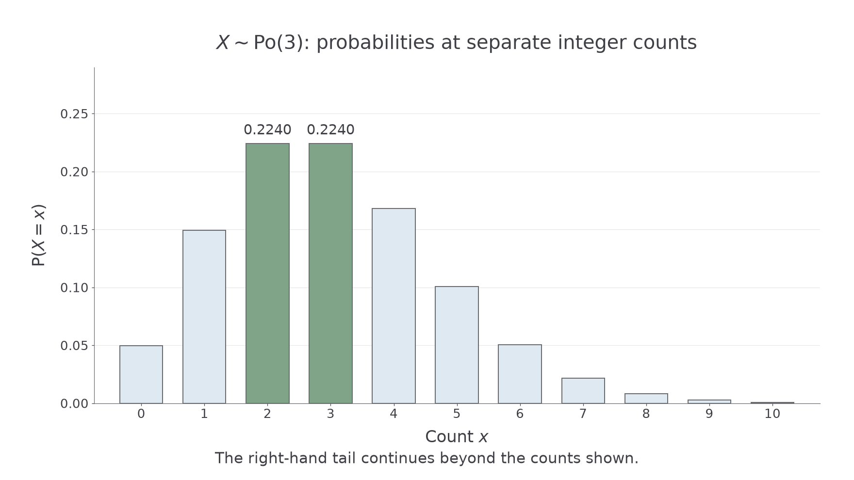
Question. Let be the number of orders in ten minutes, with . Find and , giving four decimal places.
Plan. Substitute each count into the point-probability formula and compare the exact expressions before rounding.
Why this step? Comparing the exact expressions proves equality; two rounded calculator outputs alone would not establish that the probabilities are exactly equal.
Answer. Both probabilities are to four decimal places.
Check. The ratio of consecutive probabilities here is . The opening question is answered: exactly three is not more likely than exactly two.
The bars show probabilities at separate integer counts. Their equal heights at and make the calculation visible; the right-hand tail continues beyond the counts shown.
[DIAGRAM: asset_name: Poisson point probabilities with parameter three; asset_slug: 9fm0-fs103-poisson-three; caption: With parameter three, the counts two and three have exactly equal probabilities; description: A discrete bar chart shows Poisson probabilities for counts zero to ten with parameter three. The bars at two and three are sage and both labelled 0.2240; the other bars are pale blue. The horizontal axis is labelled count x, the vertical axis is labelled P(X equals x), and a note states that the right-hand tail continues beyond ten.]
Worked example 2 reverses the information: a probability is given and the parameter is unknown. The zero-count formula makes the parameter accessible through a logarithm.
Continue this lesson.
You’re previewing NovaLearn without an account. Create a free account to read the rest.
Create free account